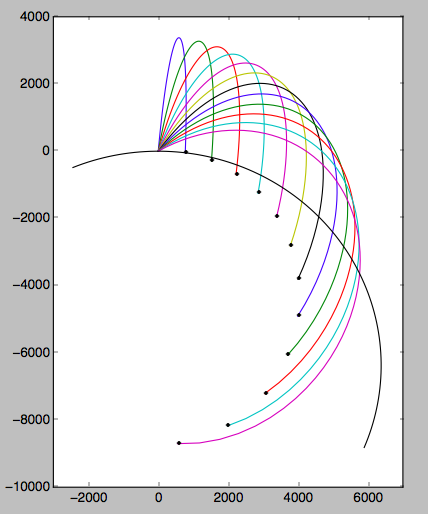
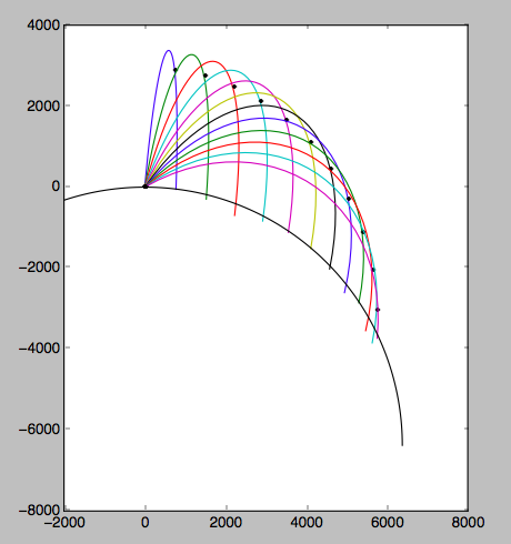
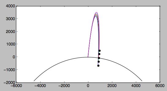
below: Simplistic simulation of a ballistic trajectory with initial velocities of 6,500 to 6,700 m/s at a small angle, with the dots representing location after 40 minutes (first plot) and 28 minutes (second plot). This is just to get a rough feeling for the scale of the trajectory and not an accurate representation of the real event, but it illustrates that the potential range of the launch is much much farther than the range of the test because the launch was nearly vertical.
def deriv(X, t):
    x, v = X.reshape(2, -1)
    acc  = -GMe * x * ((x**2).sum())**-1.5
    return np.hstack((v, acc))

import numpy as np
import matplotlib.pyplot as plt
from scipy.integrate import odeint as ODEint

GMeeightthpi, quarterpi, halfpi, pi, twopi = [2**n*np.pi for n in range(-3, 2)]
degs, rads = 180/pi, pi/180

GMe = 3.98600418E+14     # m^3 s^-2
re  = 6378000.
quarterpi, halfpi, pi, twopikms = [f*np.pi1E-03

time for= f60 in* [0np.25, arange(0.5, 1, 2]]
kms = 1E-0341)

answers = []

# v0s = np.linspace(6500, 6700, 5)
#     for v0 in v0s:

v0 = X06600.
thetas = rads =* np.arrayarange([0, re, 0.1*v05, np.sqrt(1-0.1**2)*v0]61, dtype=float5)

for theta in thetas:
 time   X0 = np.linspacehstack(0([0, 40*60re], 60[v0*f(theta) for f in [np.sin, np.cos]]))

    answer, info = ODEint(deriv, X0, time, full_output=True)
    answers.append(answer)

if 1 == 1:
    plt.figure()
    for answer in answers:
        stop = np.argmax(np.sqrt((answer.T[:2]**2).sum(axis=0)) < re-1000)
        x, y = kms*answerkms*answer[:stop+1].T[:2]
        print stop,
        plt.plot(x, y-kms*re)
        plt.plot(x[-1:]:28], y[-1:]:28]-kms*re, 'ok''.k')
    theta = np.linspace(quarterpi0, 3*quarterpihalfpi+eightthpi, 100)
    x, y = [kms*re*f(theta) for f in [np.cos, np.sin]]
    plt.plot(x, y-kms*re, '-k')
    plt.xlim(-2000, 7999)
    plt.show()


