added 682 characters in body
Source Link
uhoh
  • 151k
  • 56
  • 505
  • 1.6k

You could do numerical integration but I am sureguess you would want to avoid that. If you don't want to avoid that then let me know and I'll add links to several helpful posts. For completeness I'll add a short script at the end. It uses a standard library integrator but you can "roll your own". There are some flavors of Euler that are fast and accurate, or a variable step size RK45.

But the biggest problem with numerical integration is that it always gets worse over time!** So the series expansion or inverse solution + interpolation (see below) are preferable because they are strictly periodic - you always subtract an integer number of periods $T$ before calculation the position within one orbit!


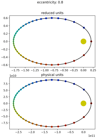
Just in case you want to get the positions by numerical integration, here's a short, simple 2D Python script to get you started. It's not meant as a solution, it just gives a "taste" of how a numerical solution would work.

numerical integration of a 2D orbit with reduced and physical units (click for full size)

Python script:

import numpy as np
import matplotlib.pyplot as plt
from scipy.integrate import solve_ivp
import time

def deriv(t, y, GM): # time derivative of state vector
    x, v = y.reshape(2, -1)
    acc = -GM * x * ((x**2).sum())**-1.5  # - GM * x_hat / abs(x)^2
    return np.hstack((v, acc))

two_pi = 2 * np.pi

e = 0.8   # eccentricity

# reduced units
GM_red = 1.   # standard gravitational parameter 
a_red = 1.   # semimajor axis

# physical units
GM_phys = 1.3271244001E+20 # m^3/s^2 (Sun) 
a_phys = 149598023000. # meters (for Earth's orbit)

# okay go for it!
names = 'reduced units', 'physical units'
semis = a_red, a_phys
GMs = GM_red, GM_phys

method = 'DOP853'
dense_output = False
n_eval = 201
tol = 1E-08

answers = []
for (a, GM, name) in zip(semis, GMs, names):
    # initialize state vector y0
    r_peri = (1 - e) * a
    v_peri = (GM * (2/r_peri - 1/a))**0.5  # https://en.wikipedia.org/wiki/Vis-viva_equation
    y0 = np.array([r_peri, 0, 0, v_peri], dtype=float)

    # initialize evaluation grid & spans (interpolator after integration finishes) 
    T_period = two_pi * (a**3/GM)**0.5 # https://en.wikipedia.org/wiki/Elliptic_orbit
    t_eval = np.linspace(0, T_period, n_eval)
    t_span = t_eval.min(), t_eval.max()

    args = (GM, )
    
    print('starting: ', name)
    t_start = time.process_time()
    print('t_span: ', t_span)
    print('y0: ', y0)
    print('args: ', args)

    answer = solve_ivp(deriv, t_span, y0, method=method, t_eval=t_eval,
                       dense_output=dense_output, events=None, args=args, 
                       atol=tol)
    answers.append(answer)
    print('finished integrating, process time (sec): ',
          time.process_time() - t_start)
    print

# okay plot the orbits
if True:
    fig, axes = plt.subplots(2, 1, figsize=[10, 6])
    ax1, ax2 = axes
    titles = 'reduced units', 'physical units'
    for answer, ax, name, title in zip(answers, axes, names, titles):
        x, y, vx, vy = answer.y
        ax.plot(x, y, '-k')
        ax.scatter(x[::5], y[::5], marker='o', c=t_eval[::5], cmap='jet')
        ax.plot([0], [0], 'oy', ms=20)
        ax.set_aspect('equal')
        difference = answer.y[:, -1] - answer.y[:, 0]
        ax.set_title(title)
    plt.suptitle('eccentricity: ' + str(e))
    plt.show()
You could do numerical integration but I am sure you want to avoid that.

You could do numerical integration but I guess you would want to avoid that. If you don't want to avoid that then let me know and I'll add links to several helpful posts. For completeness I'll add a short script at the end. It uses a standard library integrator but you can "roll your own". There are some flavors of Euler that are fast and accurate, or a variable step size RK45.

But the biggest problem with numerical integration is that it always gets worse over time!** So the series expansion or inverse solution + interpolation (see below) are preferable because they are strictly periodic - you always subtract an integer number of periods $T$ before calculation the position within one orbit!


Just in case you want to get the positions by numerical integration, here's a short, simple 2D Python script to get you started. It's not meant as a solution, it just gives a "taste" of how a numerical solution would work.

numerical integration of a 2D orbit with reduced and physical units (click for full size)

Python script:

import numpy as np
import matplotlib.pyplot as plt
from scipy.integrate import solve_ivp
import time

def deriv(t, y, GM): # time derivative of state vector
    x, v = y.reshape(2, -1)
    acc = -GM * x * ((x**2).sum())**-1.5  # - GM * x_hat / abs(x)^2
    return np.hstack((v, acc))

two_pi = 2 * np.pi

e = 0.8   # eccentricity

# reduced units
GM_red = 1.   # standard gravitational parameter 
a_red = 1.   # semimajor axis

# physical units
GM_phys = 1.3271244001E+20 # m^3/s^2 (Sun) 
a_phys = 149598023000. # meters (for Earth's orbit)

# okay go for it!
names = 'reduced units', 'physical units'
semis = a_red, a_phys
GMs = GM_red, GM_phys

method = 'DOP853'
dense_output = False
n_eval = 201
tol = 1E-08

answers = []
for (a, GM, name) in zip(semis, GMs, names):
    # initialize state vector y0
    r_peri = (1 - e) * a
    v_peri = (GM * (2/r_peri - 1/a))**0.5  # https://en.wikipedia.org/wiki/Vis-viva_equation
    y0 = np.array([r_peri, 0, 0, v_peri], dtype=float)

    # initialize evaluation grid & spans (interpolator after integration finishes) 
    T_period = two_pi * (a**3/GM)**0.5 # https://en.wikipedia.org/wiki/Elliptic_orbit
    t_eval = np.linspace(0, T_period, n_eval)
    t_span = t_eval.min(), t_eval.max()

    args = (GM, )
    
    print('starting: ', name)
    t_start = time.process_time()
    print('t_span: ', t_span)
    print('y0: ', y0)
    print('args: ', args)

    answer = solve_ivp(deriv, t_span, y0, method=method, t_eval=t_eval,
                       dense_output=dense_output, events=None, args=args, 
                       atol=tol)
    answers.append(answer)
    print('finished integrating, process time (sec): ',
          time.process_time() - t_start)
    print

# okay plot the orbits
if True:
    fig, axes = plt.subplots(2, 1, figsize=[10, 6])
    ax1, ax2 = axes
    titles = 'reduced units', 'physical units'
    for answer, ax, name, title in zip(answers, axes, names, titles):
        x, y, vx, vy = answer.y
        ax.plot(x, y, '-k')
        ax.scatter(x[::5], y[::5], marker='o', c=t_eval[::5], cmap='jet')
        ax.plot([0], [0], 'oy', ms=20)
        ax.set_aspect('equal')
        difference = answer.y[:, -1] - answer.y[:, 0]
        ax.set_title(title)
    plt.suptitle('eccentricity: ' + str(e))
    plt.show()
added 682 characters in body
Source Link
uhoh
  • 151k
  • 56
  • 505
  • 1.6k

As @ErinAnne points out high eccentricities like 0.8 are pretty dramatic and should be used with a really really low probability, otherwise your solar system will be crazy-looking and very unphysical. On astronomical timescales high eccentricity objects either get ejected or more often(more frequently?) get "calmed down" due to those weak n-body interactions with other planets.

Roughly speaking, planetary systems can, under some conditions, "cool off" over time.

You haven't mentioned masses (because you'll use only Keplerian orbits and won't do n-body) but in the thousand(s?) of known exo-planetary systems catalogued there are usually one or more often a few Jupiter-sized objects. These gravitational "moderators" (or perhaps "bullies") are constantly telling folks to "Settle down people! Find your place, take a seat" and often help planets tend towards some level of circularity.

So you can either use a series approximation for the forward problem (position as a function of time) which will converge quickly for modest eccentricities (another reason to avoid those "crazy point-eights") and need more terms for the high eccentricities, or choose and equal or unequally spaced set of angles (called eccentric anomalies in Kepler's space words) use it to get $\mathbf{r}$ and time, then interpolate that with your own daily timepoints.

(Feel free to ask a new question about the series approximations, but I think it's discussed in one Wikipedia article or another. I just can't find it right now.)

As @ErinAnne points out high eccentricities like 0.8 are pretty dramatic and should be used with a really really low probability, otherwise your solar system will be crazy-looking and very unphysical. On astronomical timescales high eccentricity objects either get ejected or more often get "calmed down" due to those weak n-body interactions with other planets.

You haven't mentioned masses (because you'll use only Keplerian orbits and won't do n-body) but in the thousand(s?) of known exo-planetary systems catalogued there are usually one or more often a few Jupiter-sized objects. These gravitational "moderators" (or perhaps "bullies") are constantly telling folks to "Settle down people! Find your place, take a seat" and often help planets tend towards some level of circularity.

As @ErinAnne points out high eccentricities like 0.8 are pretty dramatic and should be used with a really really low probability, otherwise your solar system will be crazy-looking and very unphysical. On astronomical timescales high eccentricity objects either get ejected or (more frequently?) get "calmed down" due to those weak n-body interactions with other planets.

Roughly speaking, planetary systems can, under some conditions, "cool off" over time.

You haven't mentioned masses (because you'll use only Keplerian orbits and won't do n-body) but in the thousand(s?) of known exo-planetary systems catalogued there are usually one or more often a few Jupiter-sized objects. These gravitational "moderators" (or perhaps "bullies") are constantly telling folks to "Settle down people! Find your place, take a seat" and often help planets tend towards some level of circularity.

So you can either use a series approximation for the forward problem (position as a function of time) which will converge quickly for modest eccentricities (another reason to avoid those "crazy point-eights") and need more terms for the high eccentricities, or choose and equal or unequally spaced set of angles (called eccentric anomalies in Kepler's space words) use it to get $\mathbf{r}$ and time, then interpolate that with your own daily timepoints.

(Feel free to ask a new question about the series approximations, but I think it's discussed in one Wikipedia article or another. I just can't find it right now.)

added 1144 characters in body
Source Link
uhoh
  • 151k
  • 56
  • 505
  • 1.6k

Get out your favorite "random points on a sphere" algorithm to choose these points. Their $\theta$ (similar to latitude but measured from the top of the sphere in spherical coordinates) will be the orbit's inclination, and their $phi$$\phi$ (similar to longitude) will be the orbit's longitude of ascending node.

Mathematically related and potentially interesting to Math majors dabbling in orbital mechanics for now, hopefully you'll dive in deeper!:

Get out your favorite "random points on a sphere" algorithm to choose these points. Their $\theta$ (similar to latitude but measured from the top of the sphere in spherical coordinates) will be the orbit's inclination, and their $phi$ (similar to longitude) will be the orbit's longitude of ascending node.

Get out your favorite "random points on a sphere" algorithm to choose these points. Their $\theta$ (similar to latitude but measured from the top of the sphere in spherical coordinates) will be the orbit's inclination, and their $\phi$ (similar to longitude) will be the orbit's longitude of ascending node.

Mathematically related and potentially interesting to Math majors dabbling in orbital mechanics for now, hopefully you'll dive in deeper!:

added 1144 characters in body
Source Link
uhoh
  • 151k
  • 56
  • 505
  • 1.6k
Loading
added 1144 characters in body
Source Link
uhoh
  • 151k
  • 56
  • 505
  • 1.6k
Loading
Source Link
uhoh
  • 151k
  • 56
  • 505
  • 1.6k
Loading