Flat-spin transition manoeuvre: why is the angular momentum not constant?

Question

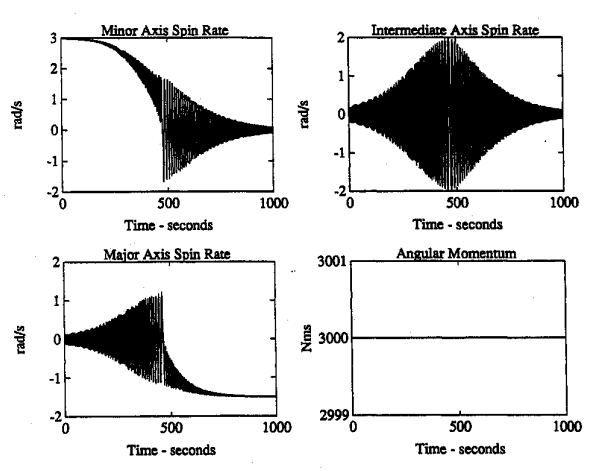
In an article by Rahn and Barba, in which a flat-spin transition manoeuvre is investigated, the following figure is presented:

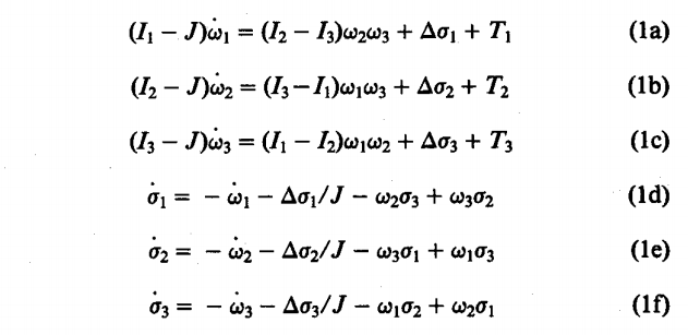
I'm trying to reproduce this figure by integrating the following coupled equations of motion stated in the article:

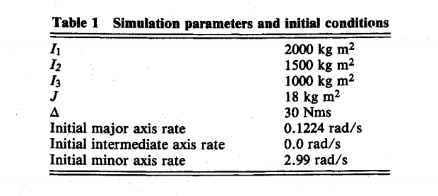
Using the following simulation parameters:

The angular momentum is calculated by:

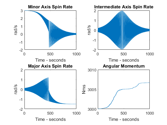
The results:

Created by the following MATLAB code:

%%%%%%%%%%%%%%%%%%%%%%%%%%%%%%%%%%%%%%%
%%%%% Example Rahn & Barba (1991) %%%%%
%%%%%%%%%%%%%%%%%%%%%%%%%%%%%%%%%%%%%%%

% Principal moments of inertia of spacecraft including slug
Ix = 2000;
Iy = 1500;
Iz = 1000;
I = [Ix Iy Iz];

% Principal moments of inertia of spherical propellant slug
J = 18;

% Spacecraft body rates
omega_x = 0.1224;
omega_y = 0;
omega_z = 2.99;
omega_0 = [omega_x omega_y omega_z];

% Relative rates between spacecraft body and propellant slug
sigma_x = 0;
sigma_y = 0;
sigma_z = 0;
sigma_0 = [sigma_x sigma_y sigma_z];

% Viscous damping coefficient
mu_x = 30;
mu_y = 30;
mu_z = 30;
mu = [mu_x mu_y mu_z];

% Torques about principal axes
Tx = 0;
Ty = 0;
Tz = 0;
T = [Tx Ty Tz];

%%%%%%%%%%%%%%%%%%%%%%%%%%%%%%%%%%%%%%%

% Integrate system of differential equations
options = [];
[t1, x1] = ode45( @omega_dynamics, [0 1000], [omega_0 sigma_0], options, I, mu, T, J );

% Calculate angular momentum
h = ((Ix * x1(:,1) + J * x1(:,4)).^2 + (Iy * x1(:,2) + J * x1(:,5)).^2 + (Iz * x1(:,3) + J * x1(:,6)).^2).^(1/2);

figure(1)
% Plot minor-axis spin rate
subplot(2,2,1);
plot(t1,x1(:,3))
axis([0 1000 -2 3])
title('Minor Axis Spin Rate')
xlabel('Time - seconds')
ylabel('rad/s')
% Plot intermediate-axis spin rate
subplot(2,2,2);
plot(t1,x1(:,2))
title('Intermediate Axis Spin Rate')
xlabel('Time - seconds')
ylabel('rad/s')
% Plot major-axis spin rate
subplot(2,2,3);
plot(t1,x1(:,1))
title('Major Axis Spin Rate')
xlabel('Time - seconds')
ylabel('rad/s')
% Plot angular momentum
subplot(2,2,4);
plot(t1,h)
title('Angular Momentum')
xlabel('Time - seconds')
ylabel('Nms')

function dx = omega_dynamics(~, x_0, I, mu, T, J)

    % Initial state vector
    omega_x = x_0(1);
    omega_y = x_0(2);
    omega_z = x_0(3);
    sigma_x = x_0(4);
    sigma_y = x_0(5);
    sigma_z = x_0(6);

    % Constants
    mu_x = mu(1);
    mu_y = mu(2);
    mu_z = mu(3);
    Ix = I(1);
    Iy = I(2);
    Iz = I(3);
    Tx = T(1);
    Ty = T(2);
    Tz = T(3);

    % Differential equations
    omega_dot_x = ((Iy - Iz)*omega_y*omega_z + mu_x*sigma_x + Tx)/(Ix - J);
    omega_dot_y = ((Iz - Ix)*omega_z*omega_x + mu_y*sigma_y + Ty)/(Iy - J);
    omega_dot_z = ((Ix - Iy)*omega_x*omega_y + mu_z*sigma_z + Tz)/(Iz - J);
    sigma_dot_x = -omega_dot_x - mu_x*sigma_x/J - omega_y*sigma_z + omega_z*sigma_y;
    sigma_dot_y = -omega_dot_y - mu_y*sigma_y/J - omega_z*sigma_x + omega_x*sigma_z;
    sigma_dot_z = -omega_dot_z - mu_z*sigma_z/J - omega_x*sigma_y + omega_y*sigma_x;

    % Return vector
    dx = [omega_dot_x; omega_dot_y; omega_dot_z; sigma_dot_x; sigma_dot_y; sigma_dot_z];

end

As can be seen from the results, the angular momentum, which should be constant, is not constant, and even increases during the transition manoeuvre. I've checked my code up and down, but could not find any mistakes. I'm guessing it has something to do with the ode45 function, but I'm not sure. Does anyone here have a clue about what's going on?

Answer 1

Short answer: it's an ODE solver issue.

When adjusting the relative and absolute error tolerances, better results are attained. For example, the options variable in the MATLAB code can be defined as follows:

options = odeset('RelTol',1e-10,'AbsTol',1e-10);

Also, to let the initial angular momentum be 3000, instead of 3000.0045 (as was pointed out in this answer), the equation for calculating the angular momentum can be solved for the initial minor axis spin rate, as follows:

omega_z = ( ( 3000^2 - ( Ix * omega_x )^2 ) / ( Iz^2 ) )^( 1/2 );

Finally, to adjust the axes of the angular momentum plot, add:

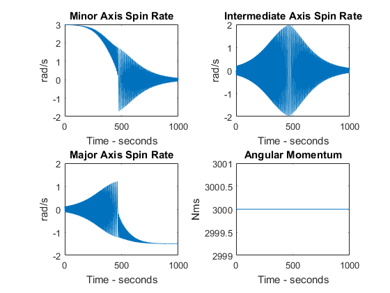
axis([0 1000 2999 3001])

This generates the following figure:

Answer 2

I rewrote your matlab into Python (which is really easy to do and that's not a coincidence!) and used the default SciPy ODE integrator. Checking info['mused'] I see that it always used the Adams (non-stiff) algorithm, so stiffness isn't the problem.

Why not just dump "Old and busted" Matlab and adopt "New hotness" Python? (MIB reference)

I would guess that you should start reading your Matlab documentation for ode45 and set your error tolerance lower. I am guessing that ode45 is what I would call RK45 and is a variable step size 4/5 order Runge-Kutta. It should be fine but if you don't specify a tolerance, it will choose one for you.

It's possible that between the time your reference was published and when you ran your example, Matlab changed some defaults or the author may have used some and forgotten to tell you, or you didn't notice them mentioned earlier in what you've been reading.

Long story short, it works for me just fine.

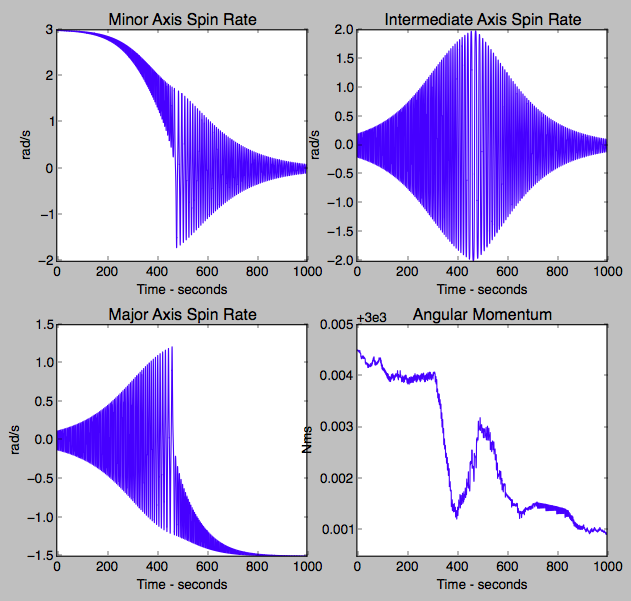
The initial angular momentum is not 3000 using the initialization values, but is actually 3000.0045which is where the simulaion starts. It drifts to 3000.001 after 1000 seconds. That's a change of 0.003. Deviation from an even 3000 (or 3e3) is shown in the plot.

I can improve that a little bit, to a total drift of only about 0.001 by inserting rtol=1E-10 or rtol=1E-11 in the call to ODEint.

def omega_dynamics(x_0, t, I, mu, T, J):

    # % Initial state vector
    omega_x, omega_y, omega_z, sigma_x, sigma_y, sigma_z = x_0[:6]

    # % Constants
    mu_x, mu_y, mu_z = mu[:3]
    Ix, Iy, Iz = I[:3]
    Tx, Ty, Tz = T[:3]

    # % Differential equations
    omega_dot_x = ((Iy - Iz)*omega_y*omega_z + mu_x*sigma_x + Tx)/(Ix - J)
    omega_dot_y = ((Iz - Ix)*omega_z*omega_x + mu_y*sigma_y + Ty)/(Iy - J)
    omega_dot_z = ((Ix - Iy)*omega_x*omega_y + mu_z*sigma_z + Tz)/(Iz - J)
    sigma_dot_x = -omega_dot_x - mu_x*sigma_x/J - omega_y*sigma_z + omega_z*sigma_y
    sigma_dot_y = -omega_dot_y - mu_y*sigma_y/J - omega_z*sigma_x + omega_x*sigma_z
    sigma_dot_z = -omega_dot_z - mu_z*sigma_z/J - omega_x*sigma_y + omega_y*sigma_x

    # % Return vector
    dx = np.array([omega_dot_x, omega_dot_y, omega_dot_z, sigma_dot_x, sigma_dot_y, sigma_dot_z])

    return dx

# %%%%%%%%%%%%%%%%%%%%%%%%%%%%%%%%%%%%%%%
# %%%%% Example Rahn & Barba (1991) %%%%%
# %%%%%%%%%%%%%%%%%%%%%%%%%%%%%%%%%%%%%%%

import numpy as np
import matplotlib.pyplot as plt
from scipy.integrate import odeint as ODEint

J        = 18.0;                                             # Principal moments of inertia of spherical propellant slug
I        = np.array([2000,   1500,   1000], dtype=float)   # Principal moments of inertia of spacecraft including slug
omega_0  = np.array([0.1224, 0,      2.99], dtype=float)   # Spacecraft body rates
sigma_0  = np.array([0,      0,      0   ], dtype=float)   # Relative rates between spacecraft body and propellant slug
mu       = np.array([30,     30,     30  ], dtype=float)   # Viscous damping coefficient
T        = np.array([0,      0,      0   ], dtype=float)   # Torques about principal axes

h_init   = np.sqrt(((I * omega_0 + J * sigma_0)**2).sum())  # % Calculate angular momentum

print "h_init: ", h_init

times        = np.linspace(0, 1000, 10001)
X0           = np.hstack((omega_0, sigma_0))

x1, info = ODEint(omega_dynamics, X0, times, args=(I, mu, T, J), full_output=True)
print x1.shape

h          = np.sqrt(((I * x1[:, :3] + J * x1[:,3:])**2).sum(axis=1))  # % Calculate angular momentum

if True:
    plt.figure()

    plt.subplot(2, 2, 1)
    plt.plot(times, x1[:, 2])
    plt.ylim(-2, 3)
    plt.title('Minor Axis Spin Rate')
    plt.xlabel('Time - seconds')
    plt.ylabel('rad/s')

    plt.subplot(2, 2, 2)
    plt.plot(times, x1[:, 1])
    plt.title('Intermediate Axis Spin Rate')
    plt.xlabel('Time - seconds')
    plt.ylabel('rad/s')

    plt.subplot(2, 2, 3)
    plt.plot(times, x1[:, 0])
    plt.title('Major Axis Spin Rate')
    plt.xlabel('Time - seconds')
    plt.ylabel('rad/s')

    plt.subplot(2, 2, 4)
    plt.plot(times, h)
    plt.title('Angular Momentum')
    plt.xlabel('Time - seconds')
    plt.ylabel('Nms')

    plt.show()