Analytical expression for the ground track of the International Space Station

Question

For a maths task in school, I am investigating the orbit of the International Space Station around the Earth. I understand that when the 3D movement in space is represented on a 2D surface, the relationship is not sinusoidal, however I have created the following (simple) model, which I am unsure is the most accurate. Below you can also find my calculated values with the formula (in red), compared to the actual values from an online API. Any help improving on this be greatly appreciated!

$$y=51.64*\sin(x-304)$$

(This only applies for one of the curves (the one pictured below), as the wave is translated 22.5 degrees to the right after each cycle.)

My data can be found in the following google doc: https://docs.google.com/spreadsheets/d/1Ac8yQn8ybdtZWK8JyKAOIw46o3UJufAoidR5unjVeHs/edit?usp=sharing

Answer 1

tl;dr: use a parametric equation.

If the Earth were not rotating, then we would have something like

\begin{align} x & = \cos \omega (t-t_0)\\ y & = \sin \omega (t-t_0) \ \cos i\\ z & = \sin \omega (t-t_0) \ \sin i\\ \end{align}

where the radius of the orbit is 1, $\omega$ is $2 \pi/T$ and $T$ is the orbital period, and $i$ is the inclination of the orbit.

Then we would have

\begin{align} lon & = \arctan2(y, x) + const\\ lat & = \arcsin(z)\\ \end{align}

If the Earth is rotating then

$$lon = \arctan2(y, x) - \omega_E (t-t_0) + const$$

where $\omega_E$ is $2 \pi/T_D$ and $T_D$ is a sidereal day (23h, 56m, 4s roughly).

Solving this for longitude as a function of latitude looks like some serious work and I am not sure there is an analytical solution.

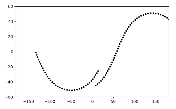
Instead you can try the parametric equation approach where you first make a hidden table of times, and then solve for $lon(t)$ and $lat(t)$ and plot $lat$ vs $lon$

Here is a plot, I haven't adjusted $t_0$ or $const$ and just used rough values for $\omega$, $\omega_E$ and $i$ but it should be enough to get you stared.

$t_0$ and $const$ represent the known starting conditions of the spacecraft that you are trying to plot; $t_0$ is the time at which it crosses the equator going north, and $const$ is the longitude on the Earth below the spacecraft at that time.

Here is some further reading:

• 5 Orbit and Ground Track of a Satellite
• Describing Orbits
• Theory of satellite ground-track crossovers

Python script:

import numpy as np
import matplotlib.pyplot as plt

twopi = 2*np.pi
to_degs, to_rads = 180/np.pi, np.pi/180.

omega = twopi/(92*60)
omega_E = twopi/(23*3600 + 56*60 + 4)

time = 60 * np.arange(101.) # 100 minutes

t0 = 1000. # arbitrary, you can fit this later
inc = 51.
const = 1.0  # arbitrary, you can fit this later

x = np.cos(omega * (time-t0))
y = np.sin(omega * (time-t0)) * np.cos(to_rads*inc)
z = np.sin(omega * (time-t0)) * np.sin(to_rads*inc)

lon = np.arctan2(y, x) - omega_E * (time-t0) + const
lat = np.arcsin(z)

if True:
    plt.figure()
    plt.plot(to_degs*lon, to_degs*lat, '.k')
    plt.xlim(-180, 180)
    plt.ylim(-60, 60)
    #plt.gca().set_aspect('equal')
    plt.show()