Calculate position of planet on fictitious orbit each day

Question

I'm a software developer but my degree with in mathematics. I'm trying to develop a game/simulation of a fictitious randomly generated solar system, and trying to work out how to model and calculate the planetary orbits. I've been reading what resources I can find and understand, especially https://calgary.rasc.ca/orbits.htm and feel I am close to what I need, but stuck on a few points at the end.

Firstly I think I can happily ignore:

• That the planet(s) orbit and the sun itself orbit around the solar system barycenter / that the gravity of the planet(s) pull on the sun. I can assume the sun is a fixed point (0,0,0) and the planets orbit around that.
• That the gravity of the planet(s) influence each other.

Given that, what I plan to do for a given random planet so far is:

1. Roll random value for "a", semi-major axis of elliptical orbit (in metres, for benefit of calculation below)
2. Roll random value for "e", eccentricity, between 0 <= e <= 0.8 seems reasonable
3. Calculate "b", semi-minor axis = a * √(1 - e²)
4. Foci are at +/- ae so can now translate the ellipse ae to the right to place one of the foci at (0,0,0) where the sun is
5. This is so far assuming the ellipse axes are lined up with the coordinate system axes so the ellipse is oriented horizontally, so now rotate the ellipse in the 2D plane a random number of degrees 0 <= r < 360 (I'm afraid I have not yet found what the correct terminology is for this)
6. Roll random value for orbit inclination, between -20 <= i <= +20 seems reasonable, and rotate the ellipse in 3D space accordingly
7. Calculate orbit duration T in seconds = 2π × √(a³ / GM) where M is the mass of the sun

Points on the ellipse can be calculated as x = a cos t, y = b sin t (then applying the translate/rotate operations in 4-6 above). So this is enough to draw the elliptical orbit. But clearly the points generated here don't take into account that the orbit is faster when the planet is closest to the sun vs its slowest when the planet is at its furthest point from the sun.

I can roll a random point on the ellipse as the starting point for the planet. But how can I calculate what point on the ellipse the planet will have each day? I see two possible approaches, I'm happy for either:

• As a definitive calculation, so a formula into which I could plug in the parameters of the ellipse and calculate coordinates for any time "t". or
• If I knew a starting point and velocity, I could simply advance the planet by that amount, and apply the effect of the sun's gravity on its velocity vector. (I wrote a simplistic demo that did just that many years ago). But this requires knowing the planet's position and direction of travel on day 1 (which I can work out as above) but also its speed to make it follow the prescribed orbit (which I do not know how to calculate, other than by a loop of guess, calculate, refine guess until I reach an acceptable level of accuracy).

Many thanks for any suggestions.

Answer 1

Wow, I think you are almost there!

Here are some goodies to get you up and running as a creator of planetary systems

2. Roll random value for "e", eccentricity, between 0 <= e <= 0.8 seems reasonable

As @ErinAnne points out high eccentricities like 0.8 are pretty dramatic and should be used with a really really low probability, otherwise your solar system will be crazy-looking and very unphysical. On astronomical timescales high eccentricity objects either get ejected or (more frequently?) get "calmed down" due to those weak n-body interactions with other planets.

Roughly speaking, planetary systems can, under some conditions, "cool off" over time.

You haven't mentioned masses (because you'll use only Keplerian orbits and won't do n-body) but in the thousand(s?) of known exo-planetary systems catalogued there are usually one or more often a few Jupiter-sized objects. These gravitational "moderators" (or perhaps "bullies") are constantly telling folks to "Settle down people! Find your place, take a seat" and often help planets tend towards some level of circularity.

So rather than a flat random distribution of eccentricity between 0 and "really high", I recommend either a normal (Gaussian) distribution centered at 0 or say 0.1, or a pseudo-thermal (exponentially decreasing) distribution of eccentricities.

• What is a thermal distribution of eccentricities?

If you'd like some suggestions how to use random number generator libraries to get truncated normal (Gaussian) distributions or thermal distributions (or others) please let me know and I'll add some here.

Or you can also ask that as a new question. You might consider Scientific Computing SE as long as perhaps you call it a "simulation" and not a "game". ;-)

---

I can roll a random point on the ellipse as the starting point for the planet. But how can I calculate what point on the ellipse the planet will have each day?

You could do numerical integration but I guess you would want to avoid that. If you don't want to avoid that then let me know and I'll add links to several helpful posts. For completeness I'll add a short script at the end. It uses a standard library integrator but you can "roll your own". There are some flavors of Euler that are fast and accurate, or a variable step size RK45.

But the biggest problem with numerical integration is that it always gets worse over time!** So the series expansion or inverse solution + interpolation (see below) are preferable because they are strictly periodic - you always subtract an integer number of periods $T$ before calculation the position within one orbit!

Instead, what's really cool to find out is that for a Keplerian orbit (elliptical or otherwise) while position as a function of time can't be calculated analytically (you need a series approximation or an integration) the inverse problem: time as a function of position - has an analytical solution! See for example:

• This answer to What is the analytical closed-form solution of the two-body problem to verify its numerical integration results?
• This answer to https://space.stackexchange.com/a/61014/12102 and references therein.

So you can either use a series approximation for the forward problem (position as a function of time) which will converge quickly for modest eccentricities (another reason to avoid those "crazy point-eights") and need more terms for the high eccentricities, or choose and equal or unequally spaced set of angles (called eccentric anomalies in Kepler's space words) use it to get $\mathbf{r}$ and time, then interpolate that with your own daily timepoints.

(Feel free to ask a new question about the series approximations, but I think it's discussed in one Wikipedia article or another. I just can't find it right now.)

For orbital inclination and longitude of ascending node

These two Keplerian orbital parameters define the plane of the orbit. The best way to generate pairs randomly in my opinion (or at least the coolest) is to appreciate that each orbital plane has a single normal vector, and they all point from your orbital center (your Sun in your scheme) to some place on a unit sphere.

Retrograde orbits (circling the "wrong way" are defined by points in the lower hemisphere of the same unit sphere.

Get out your favorite "random points on a sphere" algorithm to choose these points. Their $\theta$ (similar to latitude but measured from the top of the sphere in spherical coordinates) will be the orbit's inclination, and their $\phi$ (similar to longitude) will be the orbit's longitude of ascending node.

If you don't already have a favorite, see the algorithms, links and code in all of the answers to

• Generate a uniform distribution on the sky

Mathematically related and potentially interesting to Math majors dabbling in orbital mechanics for now, hopefully you'll dive in deeper!:

• Why are asteroids with zero orbital inclination rare?
• Can the radial oscillations of an elliptical orbit be solved using a fictitious centrifugal potential?
• Which mass distributions guarantee two bodies have non-Keplerian orbits? Which non-spherical distributions still allow noncircular Keplerian orbits? (answers incomplete - they don't fully "span the space" (humor). I should probably ask a new question in Math SE or Math Overflow.)

---

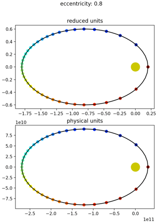
Just in case you want to get the positions by numerical integration, here's a short, simple 2D Python script to get you started. It's not meant as a solution, it just gives a "taste" of how a numerical solution would work.

(click for full size)

Python script:

import numpy as np
import matplotlib.pyplot as plt
from scipy.integrate import solve_ivp
import time

def deriv(t, y, GM): # time derivative of state vector
    x, v = y.reshape(2, -1)
    acc = -GM * x * ((x**2).sum())**-1.5  # - GM * x_hat / abs(x)^2
    return np.hstack((v, acc))

two_pi = 2 * np.pi

e = 0.8   # eccentricity

# reduced units
GM_red = 1.   # standard gravitational parameter 
a_red = 1.   # semimajor axis

# physical units
GM_phys = 1.3271244001E+20 # m^3/s^2 (Sun) 
a_phys = 149598023000. # meters (for Earth's orbit)

# okay go for it!
names = 'reduced units', 'physical units'
semis = a_red, a_phys
GMs = GM_red, GM_phys

method = 'DOP853'
dense_output = False
n_eval = 201
tol = 1E-08

answers = []
for (a, GM, name) in zip(semis, GMs, names):
    # initialize state vector y0
    r_peri = (1 - e) * a
    v_peri = (GM * (2/r_peri - 1/a))**0.5  # https://en.wikipedia.org/wiki/Vis-viva_equation
    y0 = np.array([r_peri, 0, 0, v_peri], dtype=float)

    # initialize evaluation grid & spans (interpolator after integration finishes) 
    T_period = two_pi * (a**3/GM)**0.5 # https://en.wikipedia.org/wiki/Elliptic_orbit
    t_eval = np.linspace(0, T_period, n_eval)
    t_span = t_eval.min(), t_eval.max()

    args = (GM, )
    
    print('starting: ', name)
    t_start = time.process_time()
    print('t_span: ', t_span)
    print('y0: ', y0)
    print('args: ', args)

    answer = solve_ivp(deriv, t_span, y0, method=method, t_eval=t_eval,
                       dense_output=dense_output, events=None, args=args, 
                       atol=tol)
    answers.append(answer)
    print('finished integrating, process time (sec): ',
          time.process_time() - t_start)
    print

# okay plot the orbits
if True:
    fig, axes = plt.subplots(2, 1, figsize=[10, 6])
    ax1, ax2 = axes
    titles = 'reduced units', 'physical units'
    for answer, ax, name, title in zip(answers, axes, names, titles):
        x, y, vx, vy = answer.y
        ax.plot(x, y, '-k')
        ax.scatter(x[::5], y[::5], marker='o', c=t_eval[::5], cmap='jet')
        ax.plot([0], [0], 'oy', ms=20)
        ax.set_aspect('equal')
        difference = answer.y[:, -1] - answer.y[:, 0]
        ax.set_title(title)
    plt.suptitle('eccentricity: ' + str(e))
    plt.show()