satellite ground track calculation

Question

I'm trying to calculate the ground track of an earth-orbiting satellite (Longitude, latitude) I found this handy way on the documentation but it's good when trying to find a single point what if I'm trying to find long, lati for several position points like :

is there any way to do so ??

from skyfield.api import load, wgs84, EarthSatellite

ts = load.timescale()
line1 = '1 25544U 98067A   22043.55847865  .00011256  00000-0  20676-3 0  9998'
line2 = '2 25544  51.6418 233.7857 0005922 124.4921 351.1177 15.49734813325856'
satellite = EarthSatellite(line1, line2, 'ISS (ZARYA)', ts)
print(satellite)

t = ts.now()
geocentric = satellite.at(t)

lat, lon = wgs84.latlon_of(geocentric)
print('Latitude:', lat)
print('Longitude:', lon)

Answer 1

Possibly a bit late, but it seems like you're 99% of the way there. All you need is a loop of some kind to feed timescales into the satellite.at method.

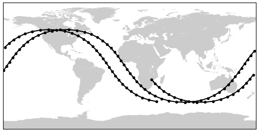
But, if you want to get a little fancy, both satellite.at and wgs84.subpoint_of can accept collections of timescales generated by ts.linspace to, for example, plot the path of the ISS every two minutes over the next 200 minutes.

import pytz
from datetime import datetime
from dateutil.relativedelta import relativedelta
from skyfield.api import load, wgs84, EarthSatellite

ts = load.timescale()

# Updated version of the listed two-line elements

line1 = '1 25544U 98067A   22078.05453850  .00006165  00000+0  11806-3 0  9995'
line2 = '2 25544  51.6427  62.9786 0003909 284.2254 162.3984 15.49468773331209'
satellite = EarthSatellite(line1, line2, 'ISS (ZARYA)', ts)
print(satellite)

# Get the current time in a timezone-aware fashion.

tz = pytz.timezone('UTC')
dt = tz.localize(datetime.utcnow())
print(f"Exectution time: {dt:%Y-%m-%d %H:%M:%S %Z}\n")

# Split the next 200 minutes into a collection of 101-evenly
# spaced Timescales (every two minutes, plus endpoints)

t0 = ts.utc(dt)
t1 = ts.utc(dt + relativedelta(minutes=200))
timescales = ts.linspace(t0, t1, 101)

# calculate the subpoints.

geocentrics = satellite.at(timescales)
subpoints = wgs84.subpoint_of(geocentrics)

# Print a nicely-formatted, tab-delimited time, latitude, and longitude.

for t, lat, lon in zip(timescales,
                       subpoints.latitude.degrees,
                       subpoints.longitude.degrees):
    print(f"{t.astimezone(tz):%Y-%m-%d %H:%M:%S}\t{lat:8.2f}\t{lon:8.2f}") 

The result will be something like this:

ISS (ZARYA) catalog #25544 epoch 2022-03-19 01:18:32 UTC
Exectution time: 2022-03-19 03:21:49 UTC

2022-03-19 03:21:49   -19.11       31.26
2022-03-19 03:23:49   -24.89       36.35
2022-03-19 03:25:49   -30.44       41.97
2022-03-19 03:27:49   -35.66       48.29
    ...

And seems like it produces a reasonable ground track when plotted on a map.

ISS Ground Track for 200 minutes following 2022-03-19 03:21: 49 UTC

This can be verified by entering the time 2022-03-19 03:21:49+0000 into the Historical ISS Tracker.

As requested by @abdalla, this is the python code using the basemap module to create the above image. I'm not too happy with the kludge I wound up using to get past basemap.plot's issues with boundary-crossing data on a cylindrical projection, but it worked in this particular instance.

import matplotlib.pyplot as plt
from mpl_toolkits.basemap import Basemap

coordinates = zip(subpoints.longitude.degrees, subpoints.latitude.degrees)

# kludge to split each crossing of the east edge of the map into its own set
# of track coordinates to route around basemap.plot rejecting the full
# coordinate set on a cylindrical projection. This code won't work for a
# westward ground track!

ground_tracks = []
prev_lon = 999
for lon, lat in coordinates:
    if lon < prev_lon:
        ground_tracks.append(([],[]))
    track_lons, track_lats = ground_tracks[-1]
    track_lons.append(lon)
    track_lats.append(lat)
    prev_lon = lon

# Create the ground track map
cyl_map = Basemap(projection='cyl', lon_0=0, lat_0=0, resolution='l')
cyl_map.fillcontinents()

# plot the individual ground tracks, then show the plot

for track in ground_tracks:
    cyl_map.plot(*track, color='black', latlon=False, marker='.')

plt.show()