What is the velocity distribution of the exhaust for a typical rocket engine?

Question

The exhaust velocity figure of a given engine is an average value. I'm curious to know how the distribution of velocities of the exhaust particles look.

From a qualitative perspective, how does the distribution typically look? Is it Normal? Lognormal? Some variation on the Boltzmann distribution? Is it multimodal due to the presence of light molecules (H₂) and heavier molecules (CO₂)? Is the standard deviation small, meaning the velocities are clustered tightly around the mean, or is it large with particle velocities spanning many orders of magnitude? Does it differ substantially between different engines or fuel types?

An example velocity distribution is below. This is what I suspect what a velocity distribution might look like - it doesn't represent any physical reality.

I know this question may be interpreted as broad, which is why I'm asking for a handwavey general answer.

Answer 1

@RussellBorogove's answer mentions temperatures of roughly 3700 K and 1800 K in the combustion chamber and exhaust of a big rocket engine.

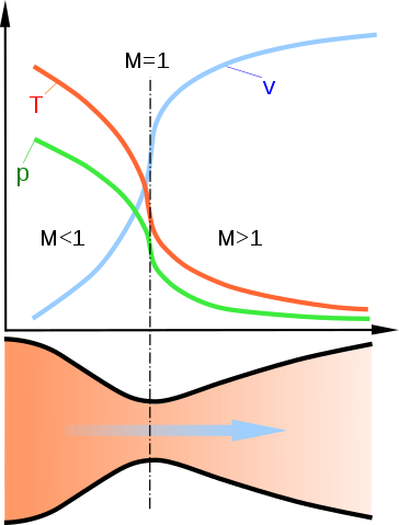
The canonical Wikipedia plot of velocity and temperature for a de Laval nozzle is shown below as a schematic representation only.

Ignoring some aspects of gas theory, we can estimate the thermal velocity of a molecule using

$$v_T = \sqrt{\frac{k_\mathrm B T}{m}}.$$

Testing example using air or nitrogen ($m=28 \times 1.673\times10^{-27}\ \mathrm{kg}$) at $293\ \mathrm K$ with Boltzmann constant $k_\mathrm B = 1.381\times 10^{-23}\ \mathrm{J/K}$ gives $297\ \mathrm{m/s}$ which does agree with the speed of sound (a good rough indicator of average thermal velocity).

species      mass (kg)      293 K     1800 K     3700 K
-------      ---------     ------     ------     ------
   H2        3.346E-27      1100       2700       3900
  CO2        7.361E-26       230        580        830

The thermal velocity will be isotropic (all directions) but the exhaust velocity is directed mostly in one direction.

The Maxwell-Boltzman distribution projected in one dimension is given as

$$f(v)\,\mathrm dv = \left( \frac{m}{2 \pi k_\mathrm B T}\right)^{1/2} \exp\left(-\frac{mv^2}{2 k_\mathrm B T}\right)\,\mathrm dv$$

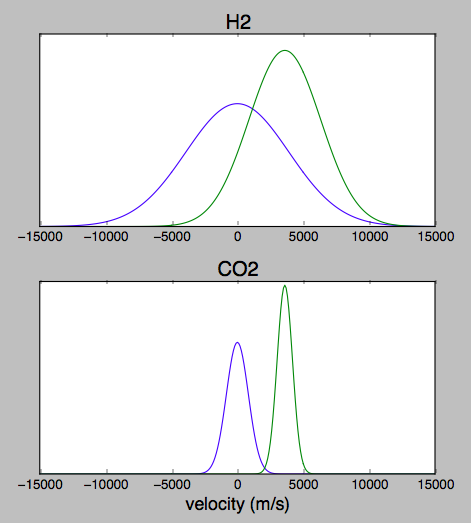
The directed exhaust velocity might be close to zero in the combustion chamber, and roughly $3600\ \mathrm{m/s}$ in the nozzle.

Assuming that the engine burns methane and a little bit of H2 is formed in the exhaust in order to fulfill the terms of the question, this plot shows the resulting estimated velocity distributions. For each species, the wide curve centered at zero represents the condition in the combustion chamber, and the narrower curve offset to the right represents the axial velocity exiting the nozzle.

The transverse velocity distribution would look similar except that the the offset for the exhaust curve would be closer to zero and depend on distance from the axis and details of under/over expansion. That's a more complicated calculation and has too many special cases for to address for this level of approximation.

def f(v, v0, m, T):
    term_1 = np.sqrt((m)/(twopi * kB * T))
    term_2 = (m * (v-v0)**2)/(2*kB*T)
    return term_1 * np.exp(-term_2)

import numpy as np
import matplotlib.pyplot as plt

twopi = 2 * np.pi
kB    = 1.381E-23
mp    = 1.673E-27

temps       = np.array([3700, 1800])
v0s         = np.array([0,    3600])
m_H2, m_CO2 = mp * np.array([2, 44])
v           = np.linspace(-15000, 15000, 301)

f_H2   = [f(v, v0, m_H2,  T)  for (T, v0) in zip(temps, v0s)]
f_CO2  = [f(v, v0, m_CO2, T)  for (T, v0) in zip(temps, v0s)]

if True:
    fig = plt.figure()
    for i, (f, name) in enumerate(zip((f_H2, f_CO2), ('H2', 'CO2'))):
        ax = fig.add_subplot(2, 1, i+1)
        # plt.subplot(2, 1, i+1)
        for thing in f:
            ax.plot(v, thing)
        ax.set_title(name, fontsize=18)
        # ax.set_yticklabels([]) # no labels
        plt.gca().axes.get_yaxis().set_visible(False) # no labels or ticks
    ax.set_xlabel('velocity (m/s)', fontsize=16)
    plt.show()

Source