How to find eccentric anomaly by mean anomaly?

Question

Wikipedia gives me the equation

M = E - e*sinE

I have M and need to find E.

How to do it?

Answer 1

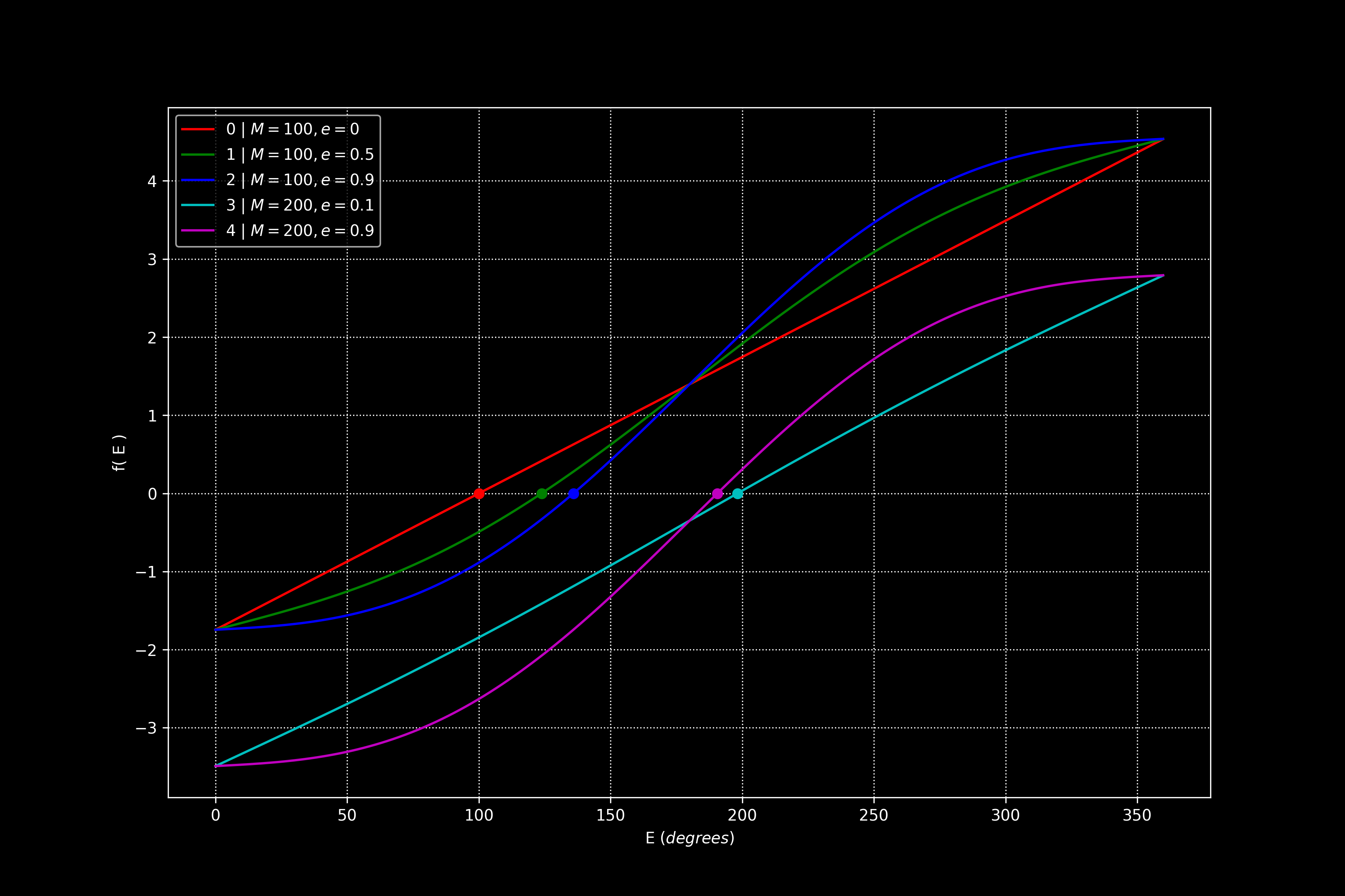
You can use a root solving method to calculate eccentric anomaly

As you stated, Kepler's equation for eccentric / mean anomaly and eccentricity is:

$M=E-e sin(E)$

and there is no closed form solution for E as a function of M but you can still iteratively calculate E.

You can set this up as a root solving problem by subtracting M from both sides of the equation to create a function that you want to find the root of (or when it equals 0 as a function of E):

$f(E)=E-esin(E)-M=0$

The root solver's solution will then calculate a value of E such that this equation equals 0, thus telling you the eccentric anomaly that satisfies Kepler's equation (the solution).

For a Newton root solver you need to calculate the derivative of this function (with respect to E), which is:

$\dfrac{d(f(E))}{dE}=1-ecos(E)$

With those two equations, values for mean anomaly (M), eccentricity (e), and an initial guess for eccentric anomaly (E) (this can be 0), the Newton root solver will calculate the solution.

As other comments stated, this only works for closed orbits (circular and elliptical), because by definition parabolic and hyperbolic orbits don't have a period. The hyperbolic eccentric anomaly is used for parabolic / hyperbolic orbits: What is hyperbolic eccentric anomaly F?

Here's a good diagram explaining mean anomaly ( https://en.wikipedia.org/wiki/Mean_anomaly ). To summarize it, mean anomaly is the "true anomaly" of an orbit with the same period as the orbit you are modeling, except it is circular, thus has a constant ("mean") angular velocity.

Here is the Python script used for making this plot. The Newton root solver can be found here: https://github.com/alfonsogonzalez/AWP/blob/main/src/python_tools/numerical_tools.py

'''
Create visualizations for Kepler's equation
of Mean / Eccentric anomalies and eccentricity
'''

from numerical_tools import newton_root_single_args
from numerical_tools import d2r, r2d

import numpy             as np
import matplotlib.pyplot as plt
plt.style.use( 'dark_background' )

def keplers_eq( E, args ):
    return E - args[ 'e' ] * np.sin( E ) - args[ 'M' ] 

def dkep_dE( E, args ):
    return 1.0 - args[ 'e' ] * np.cos( E )

if __name__ == '__main__':
    args0   = { 'M': 100 * d2r, 'e': 0.0 }
    args1   = { 'M': 100 * d2r, 'e': 0.5 }
    args2   = { 'M': 100 * d2r, 'e': 0.9 }
    args3   = { 'M': 200 * d2r, 'e': 0.1 }
    args4   = { 'M': 200 * d2r, 'e': 0.9 }
    Es      = np.arange( 0, 2 * np.pi, 0.01 )
    Es_deg  = Es * r2d
    args    = [ args0, args1, args2, args3, args4 ]
    colors  = [ 'r', 'g', 'b', 'c', 'm' ]
    labels  = [ '0 | $M=100,e=0$', '1 | $M=100,e=0.5$', '2 | $M=100,e=0.9$' ]
    labels += [ '3 | $M=200,e=0.1$', '4 | $M=200,e=0.9$' ]

    plt.figure( figsize = ( 12, 8 ) )
    for n in range( len( args ) ):
        fs   = keplers_eq( Es, args[ n ] )
        root = newton_root_single_args( keplers_eq, dkep_dE, 0.0, args[ n ] )
        plt.plot( Es_deg, fs, colors[ n ], label = labels[ n ] )
        plt.plot( root[ 0 ] * r2d, 0, colors[ n ] + 'o' )


    plt.ylabel( 'f( E )' )
    plt.xlabel( 'E $(degrees)$' )
    plt.grid( linestyle = 'dotted' )
    plt.legend()
    plt.show()

Answer 2

As the wikipedia article states, there is no closed form way to express $E$ in terms of $M$.

You would have to approximate it, for example using a series expansion:

$$E \approx M + \left(e - \frac{1}{8} e^3\right) \sin{(M)} + \left(\frac{1}{2}e^2 \right)\sin{(2M)} + \left(\frac{3}{8} e^3\right) \sin{(3M)}$$

See Morrison 1882 for details about making your own approximation.