Restricted Three body problem need to create an orbit around the two massive bodies

Question

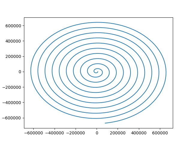
I have assignment and part of it involves getting a satellite to orbit both the Earth and the Moon at least once. How ever no matter how I set my initial condition or parameterize my position and time evolve it my satellite won't orbit the moon and comeback. Note both the Moon and Earth lie on the x axis the system is in their co-rotating frame, I am using a fourth order Runge Kutta to simulate the orbit.

Update 1: After some suggestion from the comments below my script to explain the problem a bit more when I run my code the satellite spirals out and does not orbit , I have also added a plot of the satellite

Update 2 : For those wondering where I got my acceleration term for the satellite and why it includes Coriolis and the Centrifugal force along with the gravitational force between satellite and Earth and Satellite and moon see this reference http://farside.ph.utexas.edu/teaching/336k/Newtonhtml/node123.html and chapter 7 of this http://farside.ph.utexas.edu/teaching/336k/Newton.pdf

Updated 3: Fixed an error in the position of the satellite, and a typo in the comments of the code,updated the image that corresponded to the correction in the code

from pylab import plot,show,xlabel,ylabel,cla,clf
from numpy import linspace,exp,sin,cos,zeros,array,pi ,exp



M2 = 5.972e24 # M Earth kg
M1 = 7.34767309e22 # M moon kg
G= 6.6742e-11
R=3.844e8 #m Earth-moon distance
R_e =6371e3 # Earth radius
R_m = 1737e3 # Moon radius
M_0 = ((M2 - M1)/(M2 + M1))
alpha = pi/3
omega_0 = ((G*(M2 + M1))/(R**3))**(1/2)
T_a = (2*pi)/omega_0 # System period

def dot_p(a,b):
    n= len(a)
    d=0
    for i in range(n):
        d = d+ a[i]*b[i]
    return d

def abs_v(x):
    return (dot_p(x,x))**(1/2)

r_1 = array([(M2*R)/(M2 + M1),0,0],float) # Position of Moon
r_2 = array([-(M1*R)/(M2 + M1),0,0],float) #Position of Earth
omega =  array([0,0,omega_0],float) #Angular velocity of Earth and Moon

def F(r,t):
    r1 = r[0,:] #Earth position
    vr1 = r[1,:] #Earth velocity
    r2 = r[2,:] #Moon position
    vr2 = r[3,:] #Moon velocity
    r3 = array([R*cos(t),.5*R*sin(2*t),0],float)  +r[4,:] #Satellite position Figure 8 parameterization
    vr3 = r[5,:] #Satellite velocity
    fr1 = -G*M2*(r1 -r2)/(abs_v((r1-r2))**3)
    fr2 = -G*M1*(r2 -r1)/(abs_v((r2-r1))**3) 
    fr3 = (G*M1*(r3 -r_1)/(abs_v((r3-r_1))**3)) -(G*M2*(r3 -r_2)/(abs_v((r3-r_2))**3)) +2*omega_0*array([vr3[1],-vr3[0],0],float)+ (omega_0**2)*array([r3[0],r3[1],0],float) #Gravitational interaction of Satellite with Earth, Moon, Coriolis, and Centrifugal forces
    return array((vr1,fr1 ,vr2,fr2,vr3,fr3),float)



def RungeKutta4o(g,ksi10,vksi10,ksi20,vksi20,ksi30,vksi30,a,b): #Runge Kutta 4th order
    N=1000
    M = 6    
    h = float((b-a)/N)
    t = linspace(a,b,N)
    x1 = zeros((N,3),float)
    x2 = zeros((N,3),float)
    x3 = zeros((N,3),float)
    vx1 = zeros((N,3),float)
    vx2 = zeros((N,3),float)
    vx3 = zeros((N,3),float)
    r = array((ksi10,vksi10,ksi20,vksi20,ksi30,vksi30),float)
    k1 = zeros((M,3),float)
    k2 = zeros((M,3),float)
    k3 = zeros((M,3),float)
    k4 = zeros((M,3),float)
    for i in range(N):
        x1[i,:] = r[1,:]
        vx1[i,:] = r[0,:]
        x2[i,:] = r[3,:]
        vx2[i,:] = r[2,:]
        x3[i,:] = r[5,:]
        vx3[i,:] = r[4,:]
        k1 = h*g(r,t[i])
        k2 = h*g(r +.5*k1,t[i]+.5*h)
        k3 = h*g(r +.5*k2,t[i]+ .5*h)
        k4 = h*g(r +k3,t[i]+h)
        r += (1/6)*(k1 + 2*k2 + 2*k3 + k4)
    return t,x1,x2,x3,vx1,vx2,vx3 

cla()   # Clear axis
clf()
r_i0 = r_2 + array([0,R_e+300e3,0],float) # Satellite is initially in Earth orbit
vr_i0 = array([11000,0,0],float) # Initial velocity of satellite
t,R1,R2,R3,vR1,vR2,vR3  = RungeKutta4o(F,r_1,omega,r_2,omega,r_i0,vr_i0,0,10*T_a ) 
plot(R3[:,0],R3[:,1])  #Plots the Satellite orbit R3[:,0] is the x position of the satellite and R3[:,1] is the y position of the satellite
show() 

Answer 1

What you are asking for is called a free return trajectory.

I will not be debugging your program or solving the problem for you (that's your homework), but I will pass on some advice given by Bate, Mueller & White*:

• There is more than one solution.
• Don't expect an exact solution from whatever your initial conditions may be.
• Start off by using the patched conic method.

You can then refine the approximate answer with a more exact numerical integration. If your integrator gives a wildly different answer from patched conics, try inputting some simple Earth orbits and see if the answers make sense. You can check the orbit against an analytical method for perturbations by the moon. It is likely that the integrator is buggy.

Use the patched conic approximation to get a feel for how the evolution of the system is affected by small changes in the initial conditions. Think of what happens at the patch points.

*Fundamentals of Astrodynamics, 1971, Dover, exercise 7.12 on p. 354.