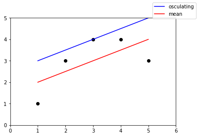
I find these terms easiest to explain using an analogy.
Let’s take these 5 points in the x,y plane:
(1,1) (2,3) (3,4) (4,4) (5,3)
We can perform the following operations on them in a Jupyter Notebook
and produce a simple plot:
%pylab inline

x = array([1, 2, 3, 4, 5])
y = array([1, 3, 4, 4, 3])
fig, ax = plt.subplots()
ax.plot(x, y, 'ko')
ax.set(xlim=[0,6], ylim=[0,5])

# Osculating elements touch the input
# curve exactly, but only in one place.
# Here we intersect point [2], with the
# slope of points [1] and [3].

dx = x[3] - x[1]
dy = y[3] - y[1]
m = dy / dx
c = y[2] - m*x[2]
print(m, c)
ax.plot(x, m*x + c, 'b', label='osculating')

# Mean elements take into account all
# the input positions, but may not
# exactly intersect any of them.

A = np.vstack([x, np.ones_like(x)]).T
m, c = np.linalg.lstsq(A, y, rcond=None)[0]
print(m, c)
ax.plot(x, m*x + c, 'r', label='mean')

fig.legend()

The code and plot illustrate four concepts:
A regression curve is any scheme
that produces a formula for not only modeling our points themselves
(with more or less accuracy, depending on the scheme)
but for extrapolating a curve
in the gaps between the points themselves.
Many such schemes are possible.
A linear regression is any scheme
that commits to using the specific regression curve y = mx + c
and that comes up with values for m and c
that somehow model the input points.
One possible (though quite primitive)
linear regression is to generate an osculating line
that (a) just barely comes tangent to the data at one point,
and (b) whose slope is determined by the two points around it.
This regression will ignore the rest of the data beyond those three points.
Another possibility is to perform ordinary least squares
to choose the line,
which tries to keep the line from straying too far from any of the data points,
but will perhaps not pass directly through any of them.
With these concepts in hand,
we can now draw sharp analogies
to the corresponding four concepts that you have asked about:
Orbital elements are, strictly speaking, any set of numbers
with an accompanying scheme that turns those numbers
into a continuous curve representing an orbit.
Keplerian elements are specifically the six parameters e, a, i, Ω, ω,
and one of the anomalies,
that when supplied to a Keplerian 2-body propagation routine
will produce a position.
Osculating elements are a set of elements
(whether Keplerian or not!)
that are specifically chosen
so that at one exact moment in a body’s real-life travel,
the elements exactly reproduce its position and velocity.
Given that the universe is an n-body problem,
never before and never again will the elements
exactly match the body’s position and velocity,
but they tend to be very good for a brief time right around that moment.
Mean orbital elements are, by contrast, a set of elements
(whether Keplerian or not!)
that are chosen to pass relatively close
to a whole series of observations of a body.
In exchange for trying to not stray too far from any of the positions,
the mean elements will not, alas, pass exactly through any of them.
In discussions of comet and asteroid orbits,
these concepts operate in a fairly pure form:
usually such bodies are modeled with strict Keplerian 2-body elements,
so that any element set for them is going to be either
an “osculating Keplerian orbit” or a “mean Keplerian orbit”.
Planetary orbits are complicated enough
that I rarely see discussion of mean elements for them.
Typically astronomers will either use a full n-body simulation
(or a JPL ephemeris that results from such a simulation run on JPL computers),
or else they will use osculating elements —
for example, to draw a planet’s orbit in a planetarium program
as a closed curve,
instead of drawing the real orbit
that never returns to the exact same place after each revolution.
Finally, earth satellite orbits are most complex,
because a set of Kepler-like parameters are supplied
to an algorithm called SGP4 —
which is a noticeably non-Keplerian attempt to model how real satellite orbits
are warped by influences like the Moon’s gravity
and by decay from atmospheric friction.
I call SGP4 merely “Kepler-like” because if you give SGP4 the orbital elements
that you would normally expect to produce a given position and velocity,
you’ll get a somewhat different position and velocity out!
Whether you want to produce osculating SGP4 elements,
or mean SGP4 elements,
you are going to have to start with approximate elements
then use an optimizer to tweak them until the output of SGP4
is either the osculating position and velocity,
or the mean solution,
that you want.
These are the strict definitions.
You will usually find that in any particular discussion or context,
any one term might imply several of the others,
depending on the community in which the discussion is taking place.
