I use a Kepler's Problem solver to test a Lambert's Problem solver. For example: if I want to generate a wide variety of test cases where I vary eccentricity and semimajor axis, I simply solve:
$$
M_0 + \sqrt{\frac{\mu}{a^3}}\Delta t = E - e \sin(E)
$$
for a wide variety of $(e, a, \Delta t)$ combinations. Having solved a multitude of Kepler's problems (which I can test immediately, because Kepler's equation must hold) I solve the corresponding Lambert's problem and verify that I obtain the same eccentric anomaly.
The following code explains this approach
import numpy as np

def kepler(a, e, mu=1.0):
    # EXPLICIT calculation of time of flight given eccentric anomaly
    # [in 0, 2 pi]
    n = np.sqrt(mu / pow(a, 3))
    E = np.linspace(0, 2 * np.pi, 360) # one point per degree
    t = (E - e * np.sin(E)) / n
    return (t, E)

def cartesian(sma, ecc, ean, mu=1.0):
    smp = sma * (1 - ecc**2)
    energy = -mu / (2 * sma)
    f = 2 * np.arctan(np.sqrt((1 + ecc) / (1 - ecc)) * np.tan(ean / 2))
    r = smp / (1 + ecc * np.cos(f))
    v = np.sqrt(2 * (energy + mu / r))
    if f < 0:
        f = 2 * np.pi + f
    return np.array([r, v, f])

# Let's test our algorithm for a given combination of sma/ecc. In a
# real test you would add more values, and you would consider multiple
# rev (you will get two solutions for most of the multirev cases)
sma = 1.0
ecc = 0.1

# this computes time of flight and eccentric anomaly NOTICE THIS IS AN
# EXPLICIT CALCULATION
tof, ean = kepler(sma, ecc)

# this transforms the quantities to cartesian vector magnitudes and
# unrestricted true anomaly (to compute transfer angle)
rvf = np.array([cartesian(sma, ecc, E) for E in ean])

r = rvf[:, 0]
v = rvf[:, 1]
f = rvf[:, 2]

# Here I'll just call my own Lambert solver (implemented in C++)
import ctypes
lib = ctypes.CDLL("libsolve.so")
vs = (ctypes.c_double * 2)()
N = len(tof)
max_diff = 0.0

# This ugly loop simply compares every staged-pairwise combination for
# SINGLE REV (you can do multiple rev as well, you just need to
# increase TOF and f to be urestricted). You would attach your own
# Lambert solver here.
for n1 in xrange(N):
    for n2 in xrange(n1 + 1, N):
        lib.solve(ctypes.c_double(1.0), # gm
                  ctypes.c_double(r[n1]), # norm of first position
                  ctypes.c_double(r[n2]), # norm of second position
                  ctypes.c_double(f[n2] - f[n1]), # angle traveled
                  ctypes.c_double(tof[n2] - tof[n1]), # time of flight
                  ctypes.byref(vs)) # output

        # compare the norm of velocities (you could decompose in
        # radial/tangential)
        diff = np.sqrt((v[n1] - vs[0])**2 + (v[n2] - vs[1])**2)

        if diff > max_diff:
           max_diff = diff

# report the maximum difference
print max_diff
Notice how you can calculate the time of flight given a range of eccentric anomalies, eccentricity, and semimajor axis. In this case I'm considering single-rev only, but the generalization is straightforward.
With the eccentric anomaly you can compute true anomaly and time of flight (the later via Kepler's equation, but you do not need to solve iteratively).
That information is used to obtain range and speed at different points in the orbit.
You can then use all those combinations of range, speed, time of flight, and transfer angle (difference in true anomaly because the orbit is Keplerian) to test your Lambert solver.
I ran a quick test with my own implementation of Gooding's algorithm and obtained a maximum difference of 8.76111591946e-14, perfectly reasonable for double-precision calculation.
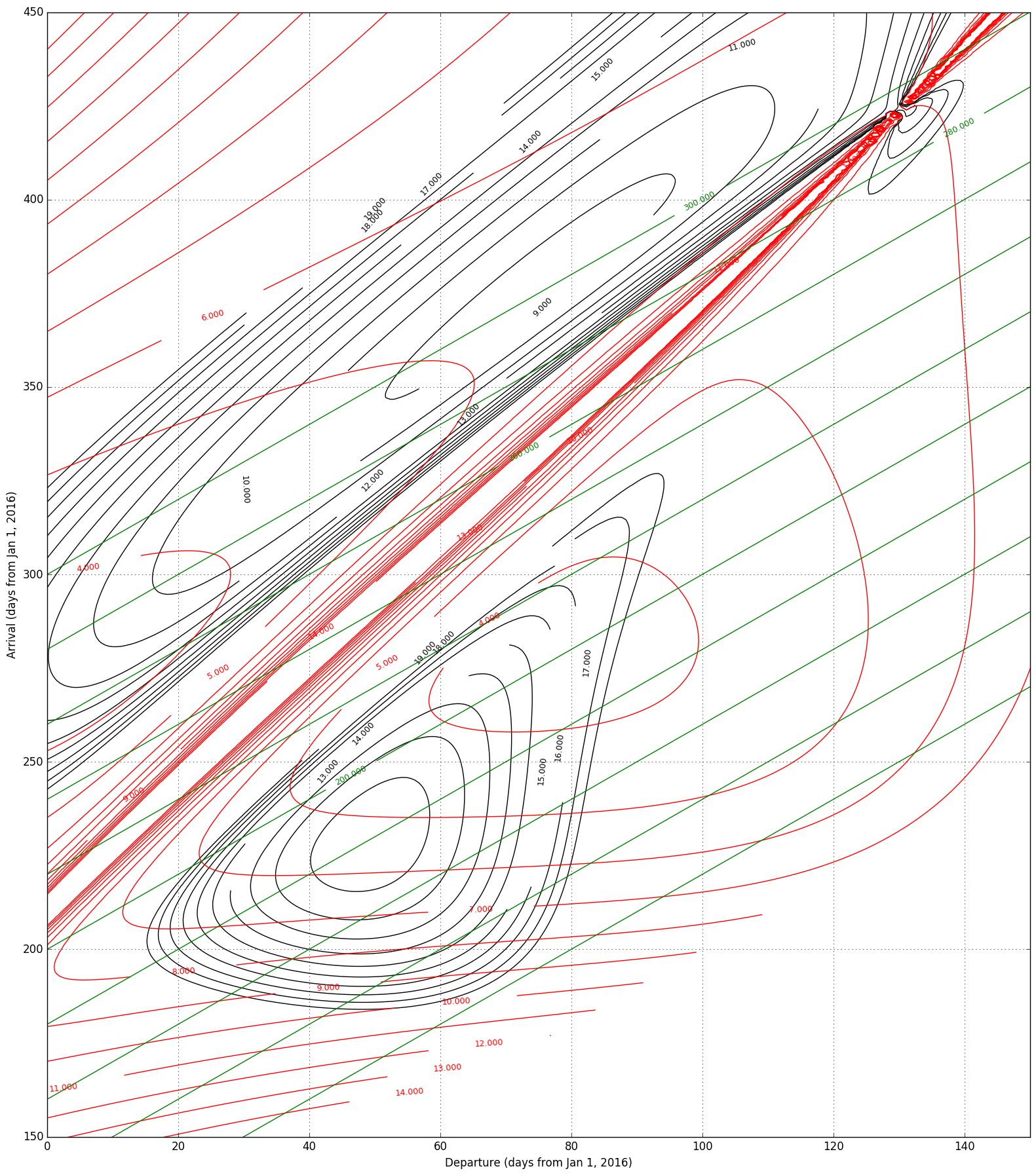
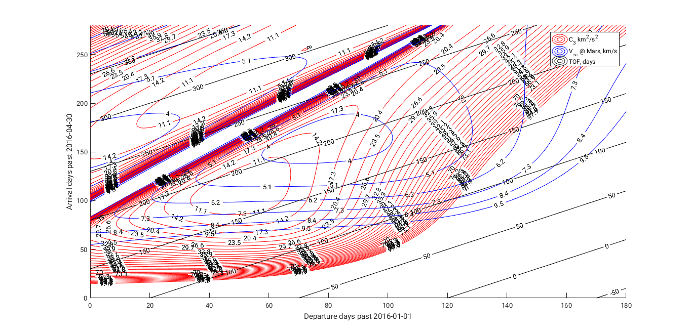
For comparison, I generated a similar diagram - it compares well with yours. I would recommend you increase the axes on your arrival time to about 420 days past Jan 01, 2016 to ensure that your Lambert solver detects the transfer node (also, please notice our different baseline epoch for our arrival dates).


