Satellite altitude as a function of time?

Question

In order to obtain a more accurate radiation estimate in this question, I am trying to approximate and/or determine the altitude of a satellite as a function of time. The satellite has an apogee of 32190 km above earth, and perigee of 320 km above earth.

I assume the following properties for simplicity:

• No orbit inclination, so in the equatorial plane,
• No J2 effects.
• No atmospheric drag/other drag forces.

If you see any mistakes please let me know :)

Approaches:

1. Find closed form analytical solution
2. Find iterative analytical solution
3. Find orbit simulation software to retrieve orbit altitude
4. Find a dataset of orbit altitudes as a function of time of equivalent satellites.

Summary of the attempt outcomes:

1. According to this attempt there is no (simple) closed form. I was trying to be effective, not to re-invent the wheel so I will switch to a numerical method to get a function of the orbit altitude.

2. Worked out in answers: The Orbital Dynamics Part 18 -- Formula for True Anomaly lecture explains how the the eccentric anomaly can be found by an iterative attempt. I was curious how this relates to the differential nature of the equation.

This solution is worked out in the answers.

3. I tried:

https://www.thanassis.space/gravity.html

http://en.homasim.com/orbitsimulation.php

https://nl.mathworks.com/matlabcentral/fileexchange/57132-satellite-orbit-transfer-simulation

The first 2 pages of these models:

http://www.winsite.com/satellite/satellite+simulator+orbit/

https://github.com/pytroll/pyorbital

And very promising but unable to download:

https://nl.mathworks.com/matlabcentral/fileexchange/57132-satellite-orbit-transfer-simulation

4. Worked out in answers: Worked, though midnight resulted in a bug, so I restarted it and awaited a half orbit (from apogee to perigee or the other way round), since symmetry yields the entire orbit. The solution is worked out in the answers.

I am not sure if this is appropriate, but thanks everyone for the critical and supportive feedback! :)

Answer 1

Approach 4 (Succesfull approach)

At this point in time, I am not able to pursue the analytical approach any further, so I found a satellite (debris) via http://stuffin.space/?intldes=2012-008N that had an orbit similar to the one I am trying to determine, wrote a small excel script that crawls the data from http://www.satview.org/forec.php?sat_id=43273U once every minute, so that tomorrow, I can sort the data and get the altitude approximation as a function of time.

The script is:

Sub absorb_data_from_vdb()
Application.Wait (Now + TimeValue("0:00:10")) 'H:MM:SS
'source: https://plus.google.com/105053415343007690451/posts/1pjy2PFVwN5
Dim ie As Object
Dim objelement As Object
Dim c As Integer
Dim i
Dim strCaptcha As String
Dim strImageSource As String
Dim img As HTMLhtmlElement 'tools =>reference Microsoft Html Object Library
Set ie = CreateObject("InternetExplorer.Application")

Dim click_changed_additions  As Integer
Dim electric_bullet_count As Integer
Dim gas_bullet_count As Integer


With ie
    .Visible = True
    .navigate "http://www.satview.org/forec.php?sat_id=43273U"
    'wait until first page loads
    Do Until .readyState = 4
        DoEvents
    Loop
    Application.Wait (Now + TimeValue("0:00:02")) 'H:MM:SS
    whole_day = 2
    Do While whole_day < 10
        .Refresh
        Do Until .readyState = 4
            DoEvents
        Loop
        Application.Wait (Now + TimeValue("0:00:02")) 'H:MM:SS

        Set elements0e = ie.document.getElementsByClassName("link_mudar") 'Get innertext to get value
        If elements0e.Length <> 0 Then
            'MsgBox (elements0e.item(2).innerText)
            elements0e.item(2).Focus
            elements0e.item(2).Click
            'MsgBox ("clicked link")
        End If

        If ThisWorkbook.Worksheets("Sheet1").Range("A1").Value - 2 < 2 Then
            ThisWorkbook.Worksheets("Sheet1").Range("A1").Value = 2
        End If
        For Iteration = ThisWorkbook.Worksheets("Sheet1").Range("A1").Value - 2 To ThisWorkbook.Worksheets("Sheet1").Range("A1").Value - 2 + 100
            Set elements0e = ie.document.getElementsByClassName("texto_track2") 'Get innertext to get value
            If elements0e.Length <> 0 Then
                ThisWorkbook.Worksheets("Sheet1").Range("A" & 2 + Iteration).Value = elements0e.item(0).innerHTML
                ThisWorkbook.Worksheets("Sheet1").Range("F" & 2 + Iteration).Value = Now()
                'MsgBox ("found from")
            End If
        Next Iteration
        For Iteration = ThisWorkbook.Worksheets("Sheet1").Range("A1").Value - 2 To ThisWorkbook.Worksheets("Sheet1").Range("A1").Value - 2 + 100
            Set elements0e = ie.document.getElementsByClassName("texto_track2") 'Get innertext to get value
            If elements0e.Length <> 0 Then
                ThisWorkbook.Worksheets("Sheet1").Range("G" & 2 + Iteration).Value = elements0e.item(1).innerHTML
                'MsgBox ("found from")
            End If
            If ThisWorkbook.Worksheets("Sheet1").Range("A1").Value < Iteration + 2 Then
                ThisWorkbook.Worksheets("Sheet1").Range("A1").Value = Iteration + 2
            End If

        Next Iteration

        proceed_boolean = False
        Do While proceed_boolean = False
        If Left(Right(Now(), 5), 2) <> Left(Right(ThisWorkbook.Worksheets("Sheet1").Range("F" & 2 + Iteration - 1).Value, 5), 2) Then
            'MsgBox ("A minute has passed")
            'MsgBox (Left(Right(Now(), 5), 2))
            'MsgBox (Left(Right(ThisWorkbook.Worksheets("Sheet1").Range("F" & 2 + Iteration - 1).Value, 5), 2))
            proceed_boolean = True
            Application.Wait Now + #12:00:02 AM# 'This waits for 5 seconds
        End If
        Loop


    Loop
End With
MsgBox ("Done")

End Sub

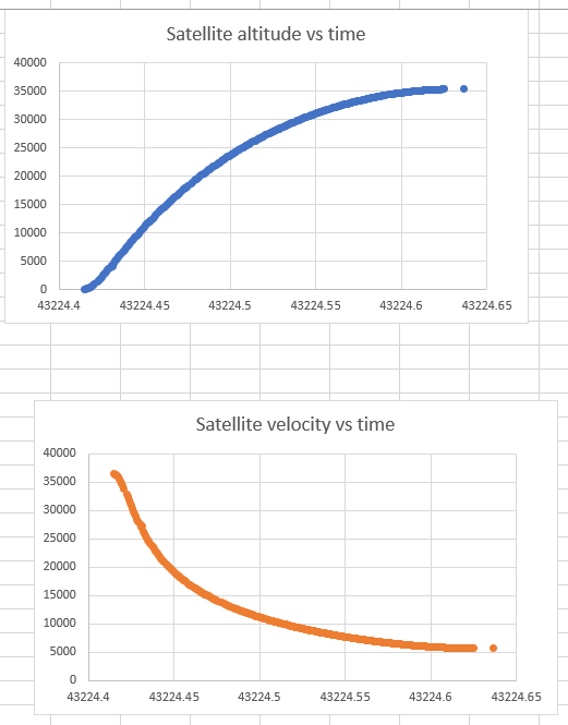
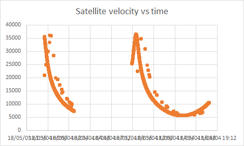
After two runs, the following graph is plotted for the equivalent orbit:

Visual inspection yields a clear orbit function, after removing the outliers. The following sanity check are performed:

1. the velocity at the perigee (lowest altitude) which should be highest, meaning the gradient of the orbit altitude function should be highest.
2. The velocity at apogee (highest altitude) should be lowest, meaning the gradient of the orbit altitude should be lowest near the perigee.
3. The gradient of the orbit altitude should equal 0 (a horizontal line at the apogee).
4. The Velocity profile is plotted separately and checked on continuity.
5. The velocity profile is plotted separately and visually checked on matching with the orbit altitude gradient.

All 5 verification are completed and successful, meaning no errors have been found in this approach.

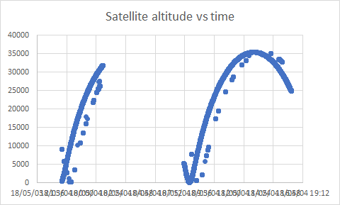
Since the orbit has an axis of symmetry only half the velocity profile is needed. As one can see, two recordings were made, the right recording contains a complete half symmetric orbit, so it yields the complete orbit altitude function after a short data manipulation. This is the orbit data that will represent the orbit altitude as a function of time, for the radiation estimation purposes.

Next the data was manually filtered (by colourmarking the magnitude of the differences between the altitude datapoints and removing the largest differences untill I was satisfied with the differences.) yielding:

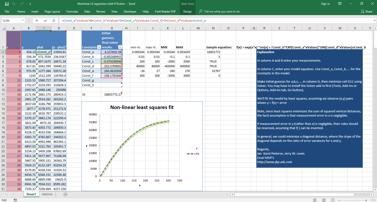
After filtering I used the following software/excel sheet to make a least squares fit: http://www.jkp-ads.com/articles/leastsquares.asp

The following polynomial function was used to approach the function**:

$y=ax^4+bx^3+c(x-f)^2+dx+e$

where x represented the time in minutes, and y was computed and compared with $y_{actual}$. The difference between the two y's was squared and summed for all datapoints (times and altitudes)scraped by the first excel). The boundary conditions (b.c.) were determined initially for the Evolutionary algorithm, by selecting the maximum value for which the highest altitude could be obtained by just that 1 coefficient multiplied by it's x, and then multiplying that value with 10. This was done to ensure the solution was obtainable, but limited the option space.

It yielded the following function**:

\begin{equation} \begin{split} const_a = 4.52765E-06\\ const_b = -0.002389915\\ const_c = -0.074298946\\ const_d = 252.5709003\\ const_e = 260.8620904\\ const_f = -108.1781644 \end{split} \end{equation}

$h(t)$ is computed in $km$ \begin{equation} h=Const_a*xValues^4+Const_b*xValues^3+Const_c*(xValues-Const_f)^2+Const_d*xValues+Const_e \label{altitude_orbit_as_func_time} \end{equation}

The Excel script can be further improved by adding an errorhandler closing the ie browser and restarting the script to ensure a higher level of automation, at the risk of greater data errors.

Error discussion: As was pointed out in the comments, the 4th degree polynomial fit will limit the accuracy of the orbit fit. (This is visible if you look at the start of the actual orbit measurement, it curves towards/around -t when going down, whereas the fitting polynomial only appears to have 1 curving radius (towards/around +t). This made the fit a bit challenging, since several iterations were required before a decent fit was found. However, this degree of accuracy was considered sufficient, by means of visual inspection. The procedure can be improved by a computation of the actual error squared.

**I think a better approach would indeed be to approximate the elliptical orbit altitude as a function of time with a sinusoidal.

Answer 2

Aproach 2 (Succesfull approach)

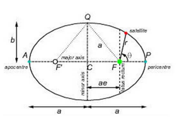
The orbit is described in the following figure:

After a long, tedious, yet wonderful derivation the following 3 equations are applicable to the elliptical orbit:

$M= \frac{t}{T}2 \pi$

$M = E-\epsilon sin{E}$

$r = a(1-\epsilon cos {E})$

$\upsilon = \theta = 2 arctan (\sqrt{\frac{1+\epsilon}{1-\epsilon}} tan{\frac{E}{2}})$

$T=2\pi\sqrt{\frac{a^3}{\mu}}$ with $\mu_{earth} = 398600.4415 \frac{{km}^3}{s^2}$

$r = \frac{a(1-e^2)}{1+e cos{\theta}} = a(1-\epsilon cos{E})$

$M(t)$ = Mean anomaly (=Angle between green line, center of ellipse, dashed line between center of ellipse and perigee)

$E(t)$ = Eccentric anomaly (=Angle between red line, center of ellipse, line between center of ellipse and perigee)

$\upsilon(t) = \theta(t)$ = True anomaly (=Angle between black line, center of ellipse, line between center of ellipse and perigee)

$a$ = semi-major axis

$r(t)$ = altitude of satellite

$\epsilon$ = eccentricity

The anomalies are visualized in the following orbit animation. Note that, as was pointed out in the comments, M(t) is constant and unequal to E(t):

Furthermore, it is necessary to compute the orbital period $T$, semi major axis $a$ and orbit eccentricity $\epsilon$ once.

Given that the perigee height = 320 km, and the apogee height 32190 km, the semi major axis is found by using $r_e = 6371 km$:

$a = \frac{320+r_e+32190+r_e}{2}= 25971.5 km$

Now the eccentricity is found using $\theta = 0 rad$:

$r = \frac{a(1-e^2)}{1+e cos{\theta}}$

$r = \frac{a(1-e^2)}{1+e} = a(1-e) $

$e =1-\frac{r}{a} = 1-\frac{r_e+320}{a} =1-\frac{6371+320}{25971.5}=0.74237144562308$

The orbital period is found with $\mu_{earth} = 398600.4415 \frac{{km}^3}{s^2}$:

$T=2\pi\sqrt{\frac{a^3}{\mu}}=41685.4 s$

So to determine the orbit at a point in time t (e.g. 0.5 $s$), the following computation steps are made for every point t at which we want to know the satellite altitude:

The mean anomaly M(t) is computed. $M= \frac{t}{T}2 \pi$

$M= \frac{0.5}{41685.4}2 \pi=0.0000753643.. rad$

Then M is substituted in:

$M = E-\epsilon sin{E}$

This leaves 1 unknown: the eccentric anomaly $E$. This is find with an iterative process (Just assume a first E, then see what you compute for $M$, check if it equals the actual computed $M$ (probably not), so then lower or increase your estimate for $E$, and see if you stray further away from $M$, or get closer to it, untill you are satisfied with the degree of accuracy of $M$, (Which implicates the degree of accuracy of $E$).

Once E(t) is determined with a sufficient degree of accuracy, it is substituded in:

$r = a(1-\epsilon cos{E})$ to find $r{t}$.

That is the orbit altitude at time t = 0.5 s. The procedure is repeated for another time t by recomputing $M(t) again.

On top of the altitude, one might also want to know the location of the satellite, relative to earth, by knowing the true anomaly. To determine the true anomaly at time t, one substitutes the iteratively found $E(t)$ in the following formula:

$\upsilon = \theta = 2 arctan (\sqrt{\frac{1+\epsilon}{1-\epsilon}} tan{\frac{E}{2}})$

This is the documentation of the procedure explained in 28:55 to 30:16 of:

.

(I did not write a script for this {iterative loop of determining/guessing $E$} (yet) so it is not semi-automated, unlike the answer of approach 4.)