How to best think of the State Transition Matrix, and how to use it to find periodic Halo orbits?

Question

I'll state my mathematical question about the state propagation and state transition matrices first, then show you a simple problem for which I would like to use these concepts to generate a densely spaced family of halo orbits.

I'll also preface with the statement that I'm looking for an Aha! type answer. I am not hoping for an explanation as long as this excellent, intuitive explanation of quaternions. I don't need everything worked out, just some explanation how one would go about understanding, getting, and using the State Transition Matrix in this context.

---

---

The following is fairly standard, I'm quoting from a paper I happen to have handy at the moment, Juan Senent, Cesar Ocampo, and Antonio Capella; Low-Thrust Variable-Specific-Impulse Transfers and Guidance to Unstable Periodic Orbits. Journal of Guidance, Control, and Dynamics, 28 (2) March–April 2005:

For the dynamical system

$$\mathbf{\dot x} = \mathbf{f}(\mathbf{x})$$

evaluated from $t_0=0$ to some $t=t_f$, the final state differential at $t_f$ is given by

$$\text{d} \mathbf{x}_f = \mathbf{\Phi}(t_f, t_0) \delta \mathbf{x}_0 + \mathbf{\dot x}_f \text{d} t_f$$

where the state transition matrix satisfies

$$\mathbf{\dot \Phi} (t,t_0) = \mathbf{F}(\mathbf{x}(t)) \mathbf{\Phi}(t, t_0) $$

and

$$\mathbf{\Phi} (t_0, t_0) = \mathbf{I}_{6 \times 6} $$

and $\mathbf{F}$ is the Jacobian of the vector field used as the state propagation matrix,

$$\mathbf{F}(\mathbf{x}(t)) = \frac{\partial\mathbf{f}(\mathbf{x})}{\partial \mathbf{x}}$$

---

I've started with the classic paper written by Kathleen Connor Howell Three-Dimensional, Periodic 'Halo' Orbits Celestial Mechanics 32 (1984) 53-71. It describes a technique to find solutions for halo orbits in the the Circular Restricted 3-body Problem (CR3BP), closely following a technique described by Breakwell, J. V. and Brown, J. V.: 1979, The "Halo" Family of 3-Dimensional Periodic Orbits in the Earth-Moon Restricted 3-Body Problem Celest. Mech. 20, 389.

Howell 1984 describes in detail a step-by-step procedure to find members of a family of halo orbits about the Lagrange co-linear libration points which have symmetry about the x-z plane, by taking advantage of the fact that for this group of orbits three of the six components of the state vector should converge to zero at the point where the orbit intersects the plane.

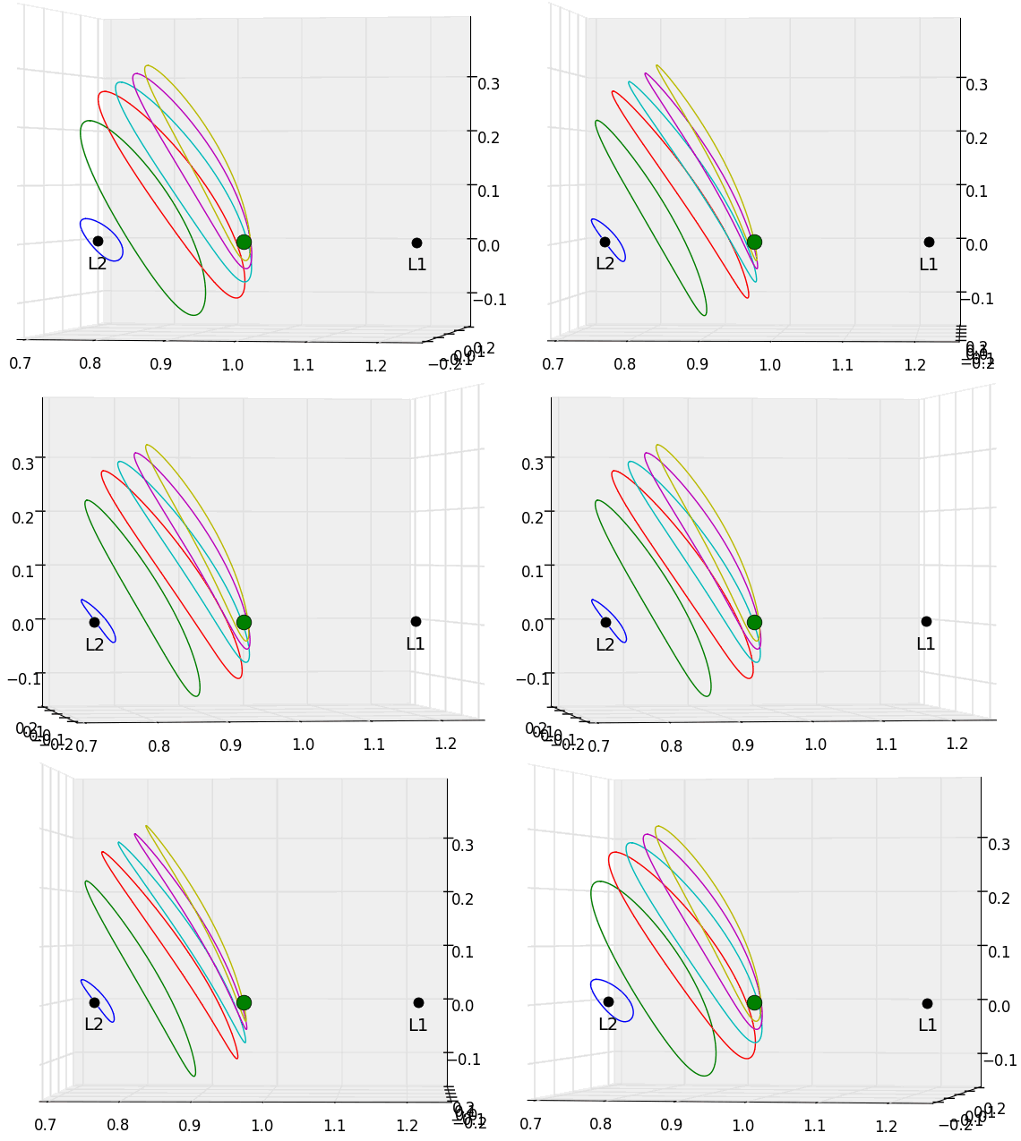
The paper tabulates six examples of halo orbits, and with the numbers given there I can integrate the state vectors, verify that the three state vector components $y, v_x, v_z$ do indeed pass through zero at the midpoint of the orbits, and make a nice plot.

What I would like to do is to understand intuitively what is a state propagation vector and a state transition vector, and how to use these to converge faster on a new member of the halo orbit family than if I had just started shooting orbits in a cluster around a starting point and used something simple like steepest descent to find the next orbit with $y, v_x, v_z$ all equal to zero.

$$\ddot{x}=x+2\dot{y}-\frac{(1-\mu)(x+\mu)}{r_1^3}-\frac{\mu(x-1+\mu)}{r_2^3}$$

$$\ddot{y}=-2\dot{x}+y\left( 1-\frac{1-\mu}{r_1^3} -\frac{\mu}{r_2^3}\right)$$

$$\ddot{z}=-z\left( \frac{1-\mu}{r_1^3} + \frac{\mu}{r_2^3} \right) $$

where

$$r_1=\sqrt{(x+\mu)^2 + y^2 + z^2}$$

$$r_2=\sqrt{(x-1+\mu)^2 + y^2 + z^2}$$

---

NOTE! I believe that the labels for the positions of L${}_1$ and L${}_2$ in the GIF and script are transposed (incorrect labels/names). I'll update the image soon.

def deriv(X, t):
    x, y, z, xdot, ydot, zdot = X
    r1 = np.sqrt((x      + mu)**2 + y**2 + z**2)
    r2 = np.sqrt((x - 1. + mu)**2 + y**2 + z**2)

    term_1 = x + 2. * ydot
    term_2 = -(1.-mu) * (x + mu) / r1**3
    term_3 =     -mu  * (x - 1. + mu) / r2**3
    xddot  = term_1 + term_2 + term_3

    term_1 = -2. * xdot
    term_2 = 1. - (1.-mu)/r1**3 - mu/r2**3 
    yddot  = term_1 + y * term_2

    term_1 = (1. - mu)/r1**3 + mu/r2**3  # should be plus???
    zddot  = -z * term_1

    return np.array([xdot, ydot, zdot, xddot, yddot, zddot])


class Sat(object):
    def __init__(self, X0, T0, nu12):
        self.X0 = X0
        self.pos0 = X0[:3]
        self.v0   = X0[3:]
        self.T0 = T0
        self.nu1, self.nu2 = nu12       


import numpy as np
import matplotlib.pyplot as plt
from scipy.integrate import odeint as ODEint
from mpl_toolkits.mplot3d import Axes3D

# From "Three-Dimensional, Periodic 'Halo' Orbits,
# Kathleen Connor Howell, Celestial Mechanics 32 (1984) 53-71 

pi, twopi = np.pi, 2*np.pi
mu = 0.04

# starting points:
x0     =   [0.723268, 0.729988, 0.753700, 0.777413, 0.801125, 0.817724]
y0     = 6*[0.0]
z0     =   [0.040000, 0.215589, 0.267595, 0.284268, 0.299382, 0.313788]
xdot0  = 6*[0.0]
ydot0  =   [0.198019, 0.397259, 0.399909, 0.361870, 0.312474, 0.271306]
zdot0  = 6*[0.0]

# X0s    = np.array(zip(x0, y0, z0, xdot0, ydot0, zdot0)) Nope! 
X0s    = np.array(list(zip(x0, y0, z0, xdot0, ydot0, zdot0)))

Thalf0s = [1.300177, 1.348532, 1.211253, 1.101099, 1.017241, 0.978653]
T0s     = [2.0*x for x in Thalf0s]

nu1s    = [1181.69,    51.07839,  4.95816,  1.101843,  0.94834,  1.10361]
nu2s    = [   0.98095, -0.90203, -0.40587, -0.420200, -1.58429, -2.09182]
nu12s   = zip(nu1s, nu2s)

n_half  = 200
fractional_times  = np.linspace(0.0, 1.0, 2*n_half+1)

rtol, atol = 1E-12, 1E-12

sats   = []
for X0, T0, nu12 in zip(X0s, T0s, nu12s):
    sat = Sat(X0, T0, nu12)
    sat.n_half  = n_half
    sat.t = sat.T0 * fractional_times
    sat.rtol, sat.atol = rtol, atol    
    sats.append(sat)

for sat in sats:
    answer, info = ODEint(deriv, sat.X0, sat.t,
                          rtol=sat.rtol, atol=sat.atol,
                          full_output = True )
    sat.answer   = answer
    sat.mid    = answer[sat.n_half]
    sat.mid    = answer[sat.n_half]
    sat.info     = info

if 1 == 1:
    xL2, xL1 = 0.74091, 1.21643  # lazy!
    fig = plt.figure(figsize=[10, 8])
    ax = fig.add_subplot(1, 1, 1, projection='3d')

    for sat in sats:
        x,  y,  z  = sat.answer.T[:3]
        ax.plot(x, y, z)

    ax.plot([0.0-mu], [0], [0], 'ob', markersize=20)
    ax.plot([1.0-mu], [0], [0], 'og', markersize=12)
    ax.plot([xL2], [0], [0], 'ok', markersize=8)
    ax.plot([xL1], [0], [0], 'ok', markersize=8)

    ax.set_xlim(0.7, 1.25)
    ax.set_ylim(-0.225, 0.225)
    ax.set_zlim(-0.15, 0.40)
    ax.text(xL1, 0, -0.05, "L1", fontsize=14, horizontalalignment='center')
    ax.text(xL2, 0, -0.05, "L2", fontsize=14, horizontalalignment='center')

    nplot    = 80
    thetas   = np.linspace(0, twopi, nplot+1)[:-1]
    azimuths = -90 + 10.0 * np.cos(thetas)

    fnames = []
    for i, azim in enumerate(azimuths):
        fname = "haloz_3D_" + str(10000+i)[1:]
        ax.elev, ax.azim = 0, azim
        plt.savefig(fname)
        fnames.append(fname)

    # tight cropping
    for i in range(len(fnames)):
        fname_in  = "haloz_3D_" + str(10000+i)[1:]
        fname_out = "haloz_3D_crop_" + str(10000+i)[1:] + ".png"
        img = plt.imread(fname_in + ".png")
        plt.imsave(fname_out, img[200:-175, 240:-190])

Answer 1

The State Transition Matrix (STM)

The STM is a linearization procedure of a dynamical system. It can be used for any non-linear dynamical system and is used to approximate the dynamics of a system over short period of times. In astrodynamics, it is used especially for statistical orbit determination (stat OD) and the circular restricted third body problem (CRTBP).

Computing the STM for stat OD is explained in depth in "Statistical Orbit Determination" by Tapley, Schultz, Born, Elsevier 2004. Specifically, section 1.2.5 and 4.2.1. From here on in, this reference will be referred to as "(1)". A posteriori reference is the state transition matrix page of the Nyx Space documentation.

System dynamics

Let $\boldsymbol{X}$ be the state of your system in a Cartesian frame. In the following, $\bf{r}$ and $\bf{v}$ respectively correspond to the position and the velocity of the spacecraft; $\dot\gamma$ corresponds to the time derivative of the $\gamma$ variable. Choosing position and velocity is often what you'll use for entry-level problems. If doing more serious stat OD, you'll also want to add in the gravitational parameter, the position of your ground stations, etc. but it's important to note that changing your state vector will also change the STM and the A matrix (cf. below).

$$\boldsymbol{X}=\left[\begin{array}{c} \boldsymbol{r}\\ \boldsymbol{v} \end{array}\right]=\left[\begin{array}{c} x\\ y\\ z\\ \dot{x}\\ \dot{y}\\ \dot{z} \end{array}\right]$$

We can then express the time derivative of the state $\boldsymbol{X}$ as follows:

$$\boldsymbol{\dot{X}}=\left[\begin{array}{c} \boldsymbol{\dot{r}}\\ \boldsymbol{\dot{v}} \end{array}\right]=\left[\begin{array}{c} \dot{x}\\ \dot{y}\\ \dot{z}\\ \ddot{x}\\ \ddot{y}\\ \ddot{z} \end{array}\right]=F\left(\boldsymbol{X}, t\right)$$

In this formulation, the $F$ function corresponds to the full dynamics of the system: this function is integrated over a period of time if you are computing the real dynamics, i.e. it is a representation of the equations of motion. Assuming the two-body problem, $\boldsymbol{\dot{v}}$ is the acceleration due only to the primary body, i.e. $-\frac{\mu}{r^3}\boldsymbol{X}$. If modeling more complex dynamics, the $F$ function will also include these.

Purpose of the STM

As said above, the STM is a linearization of your dynamics. So we start by discretizing the time and assuming that the system behaves in a linear fashion during that time. This is a very useful approximation. In fact, it allows to simplify the simulation: instead of having to propagate your dynamics (i.e. the $F$ function) over a given integration time, you simply need to multiply the state $X_{i-1}$ with the STM $\Phi$ in order to get $X_i$. Moreover, as per (1), the STM has the following properties (section and page number shown on first line for reference):

Computing the STM

So as of now, we know that the STM is a linearization of a dynamical system which allows us to consider it as a linear system over a short period of time. So, we need to linearize the dynamics of the system around a given state, herein reference. This reference is based on the time, and is updated via the STM. In other words, we compute the initial STM, compute the state at the next time, and then re-compute the STM around that new state.

The following is an extract from a lecture by Dr. McMahon. What is marked with a star corresponds to the reference state.

We can clearly see here that we're simply computing the Taylor series of the $F$ function at the first order! So mathematically this is simple. However, in practice, this corresponds to the derivative of the acceleration, so it is a bit annoying to compute (but Mathematica or Sage Math (now CoCalc) can help a bunch with their symbolic derivatives, this might help). Anyhow, this partial is generally referred to as the $A$ matrix (at least in my experience).

Relation between A matrix and the STM, from "Analysis of the Sun-Earth Lagrangian environment for the New Worlds Observer (NWO)", Deccia 2017 (link)

I think a good example is looking at how this can be done in code (these are from my astrodynamics library which is in Golang, sorry... I think/hope it's still relatively readable). Firstly, the computation of the A matrix with a number of possible perturbations based on the mission configuration. Secondly, a series of test cases. Among other things, the test checks that the norm of the difference between the previous state and the new state (computed via the STM) is within $0.1$ (this is somewhat arbitrary but the state has positions and velocities of a LEO spacecraft, so this is tiny difference). Thirdly, you may wish to check the code source of GMAT (which I have made available on Github for convenience -- check their sourceforge repository for the latest updates).

Halo Orbits and the STM

From your question, it seems you already know Halo orbits, so I won't dive into these (I'm no expert in them anyway, so I might say wrong things). In short, Halo orbits a quasi-periodic orbits around libration points (they are periodic in the CRTPB). Libration points are equilibrium points between two massive bodies. In effect, an orbit will be periodic for a given time $T$ (and therefore be a Halo orbit) if and only if at half of its period, the motion (i.e. the velocity) of the spacecraft is zero in all but one direction. This handout by Dr. Davis (of CCAR at CU Boulder) on finding Halo orbits from an initial guess details how to program this. I will add the following clarifications:

• All computations are done after a normalization between both bodies
• This solves the Halo orbits only in the circular restricted three body problem. In other problem settings, this method may not apply as such, or at all.
• $T/2$ corresponds to the half-period time
• The STM is integrated between time zero and time $T/2$: this is the whole of the discretization period. (If coming from a stat OD background, this time is much much larger than what you would use).
• The single shooting method allows to find orbits which have at least one period. Halo orbits are unstable by nature, so it is likely that propagating the "final" Halo orbit makes it diverge after more than one orbit (cf. figure below).

Answering your question (hopefully)

Why do you want to use the STM to find Halo orbits instead of brute-forcing everything?

1. Brute forcing is rarely a good idea. It is slow because it looks for all possible solutions. It depends entirely on your dicretization of the solution space. Imagine you set the step size to be 0.5 in the position of the normalized frame but the solution is actually at a 0.2 increment, then your method will never converge.
2. The STM allows to perform several iterations which are getting closer and closer to the Halo orbit. You should expect the algorithm to converge in less than 5-6 iterations (that's nothing compared to a brute force).
3. You refer to a steepest descent. I believe this would involve a gradient descent method for finding global solutions to optimization problems. Gradient descent could be applied to the STM, but it cannot work with the full dynamics (the system is not linear). In addition, a gradient descent method is applicable to convex problems, but your problem isn't necessarily convex (I don't think it is at all to be honest): you may not find a solution. So you'd have to find a dual problem which is convex, and solve the dual problem. But converting to the dual problem would be very complicated given that you have a non-linear system. Finally, and more importantly than all the math stuff above, what would be the cost function you're minimizing? Where is the optimal problem?

Code?

Disclaimer: I have not validated this Matlab code. It may be buggy, have edge cases, break down in specific cases, etc, etc. But, it may help to get an idea on how to implement this: unvalidated code. (I think I've included all the files needed to run this, but if I haven't, let me know in the comments and I'll add it -- I have no problem sharing my code, quite the contrary)

Answer 2

Let's have a try! To keep it simple, I will consider a one-dimensional equation of motion

$$m \ddot{x(t)} = a(t) x(t) + b(t) \dot{x}(t) \tag{1}$$

The applications to halo orbit is actually simpler because the coefficients $a(t)$ and $b(t)$ would not depend on time.

The theory of linear differential equations tells us two important results:

1. Initial conditions $x(0)=x_0,\ \dot{x}(0)=\dot{x}_0$ completely fix the solution;
2. Any linear combination of two solutions is also a solution.

The first result implies that there must exists a function which maps $(x_0,\dot{x}_0)$ onto $x(t)$. The second result guarantees that this function is linear, i.e.

$$ x(t) = \alpha(t)x_0 + \beta(t)\dot{x}_0$$

But then the speed has the same form

$$ \dot{x}(t) = \dot{\alpha}(t)x_0 + \dot{\beta}(t)\dot{x}_0$$

and we can therefore put everything together

$$\begin{pmatrix} x(t) \\ \dot{x}(t) \end{pmatrix} = \underbrace{\begin{pmatrix} \Phi_{11}(t,t_0) & \Phi_{12}(t,t_0) \\ \Phi_{21}(t,t_0) & \Phi_{22}(t,t_0) \end{pmatrix}}_{\displaystyle\Phi(t,t_0)} \begin{pmatrix} x_0 \\ \dot{x}_0 \end{pmatrix} \tag{2}$$

And $\Phi(t,t_0)$ is called the transition matrix from time $t_0$ to time $t$.

From this equation, since $x(t)$ satisfies the differential equation (1) we started from, we can reasonably expect $\Phi(t,t_0)$ to satisfy one too. To find it, we just need to differentiate (2)

$$\begin{pmatrix} \dot{x}(t) \\ \ddot{x}(t) \end{pmatrix} = \dot{\Phi}(t,t_0)\begin{pmatrix} x_0 \\ \dot{x}_0 \end{pmatrix}\tag{3a}$$

where $\dot{\Phi}(t,t_0)$ denotes the differentiation with respect to $t$, keeping $t_0$ constant. But then the left-hand side reads

$$\begin{pmatrix} \dot{x}(t) \\ \ddot{x}(t) \end{pmatrix} = \underbrace{\begin{pmatrix} 0 & 1\\ \frac{1}{m}a(t) & \frac{1}{m}b(t) \end{pmatrix}}_{A(t)}\begin{pmatrix} x(t) \\ \dot{x}(t) \end{pmatrix}$$ Then we use (2) to replace $\begin{pmatrix} x(t) \\ \dot{x}(t) \end{pmatrix}$ on the right-hand side. $$\begin{pmatrix} \dot{x}(t) \\ \ddot{x}(t) \end{pmatrix} =A(t)\Phi(t,t_0)\begin{pmatrix} x_0 \\ \dot{x}_0 \end{pmatrix} \tag{3b}$$

By equating the right-hand side of (3a) and (3b), we get

$$\dot{\Phi}(t,t_0)\begin{pmatrix} x_0 \\ \dot{x}_0 \end{pmatrix} = A(t)\Phi(t,t_0)\begin{pmatrix} x_0 \\ \dot{x}_0 \end{pmatrix}$$

This equality must be true for any $x_0$ and any $\dot{x}_0$. Thus the matrices acting on $\begin{pmatrix} x_0 \\ \dot{x}_0 \end{pmatrix}$ on both side of the equation shall be equal, and we get the differential equation we sought,

$$\dot{\Phi}(t,t_0) = A(t)\Phi(t,t_0). \tag{4}$$

After writing all that, I feel I have to explain the last trick in the Howell paper. So we have $x(t)$ and we want to understand what could make it vary a tiny bit. $x(t)$ depends on $t$, so varying $t$ by $\delta t$ induces a variation, proportional to the derivative: $\dot{x}(t)\delta t$. But $x(t)$ also depends on $x_0$ and $\dot{x}_0$ and that dependence is given by (2). The second row of the matrix to be exact, and the variation is $\Phi_{21}(t,t_0)\delta x_0 + \Phi_{22}(t,t_0)\delta \dot{x}_0$. Then if we consider only small variations, we can just sum those two contributions and get:

$$\delta \dot{x}(t) = \Phi_{21}(t,t_0)\delta x_0 + \Phi_{22}(t,t_0)\delta \dot{x}_0 + \dot{x}(t)\delta t$$

In the problem of interest to you, $t$ is the half-period $T/2$, and the variation $\delta \dot{x}(T/2)$ comes either from a small variation of $T/2$, for the same initial conditions, or from a small variation of the initial conditions, for the same half-period.

I hope it bring some enlightenment and I wish you the best for your project!

Answer 3

I'll try answering your two questions simply first. If these responses are too simple or miss the mark, let me know, and I'll edit the response.

1) What are the state propagation vector and State Transition Matrix (STM)?

The state propagation vector is simply the position & velocity at a given time.

The STM is a matrix that captures the sensitivity of the propagation to the initial state. So, it answers the question "If I change my starting x-coordinate by 5 meters, how much will my final position and velocity change?"

2) How can I use the STM to improve convergence on new Halo Orbits?

You can use the STM to achieve faster convergence on new Halo orbits by mapping the change you need at the Y-axis crossing back to the starting state. (E.g. if you arrive at the crossing with a +2 Z velocity, you can use the STM to compute a different initial state that will have a Z velocity reduced by about 2. (subject to linearization errors) Dr. Davis from CU Boulder (CCAR) provides the following handout in the Interplanetary Mission Design grad-course she teaches:

http://ccar.colorado.edu/imd/2015/documents/SingleShootingHandout.pdf

More over, here is the summary of a project on Halo orbits which includes a number of useful figures: http://ccar.colorado.edu/asen5050/projects/projects_2012/dowling/introduction.html