12
$\begingroup$

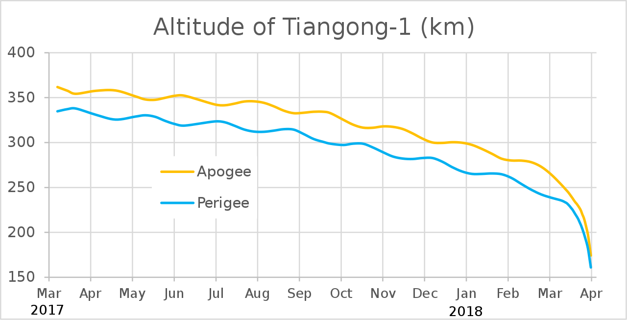
The apogee and perigee graph of the Tiangong-1 space station, about to re-enter and break up Real Soon Now, is depicted in this graph (source: Wikipedia):

Altitude of Tiangong-1

Why are the graphs wobbly? Is it because the Earth is not exactly a sphere and also due to uneven mass distribution? Is it an atmospheric effect? (Probably not a day/night issue, since the period is about 50 days).

$\endgroup$
2
  • 3
    $\begingroup$ Wild speculation here, but one possibility is that this is an aliasing artifact (from higher frequency variation, like that due to eccentricity) caused by down-sampling without proper prior filtering of the input signal. Especially if it was then subsequently plotted with a "smooth" plot, this would interpolate and render what appears to be a low-frequency oscillation. $\endgroup$
    – Dan Bryant
    Commented Apr 2, 2018 at 16:03
  • 1
    $\begingroup$ Thanks for the edit and showing me the uninterruptable single space character! I saw your profile, folliwing links there led to a company which led to OSIRIS which led me to post Yet another OSIRIS! Has the DLR/GOM Space test of the cubesat optical communications link happened yet? $\endgroup$
    – uhoh
    Commented Oct 20, 2018 at 10:53

3 Answers 3

10
$\begingroup$

Is it because the Earth is not exactly a sphere and also due to uneven mass distribution?

Yes!

Is it an atmospheric effect?

No.

Earth's large J2 or oblateness term is always trying to perturb satellite orbits, and the effect is strongest in LEO.

In this answer for example, I show how J2 constantly advances the argument of perigee of an elliptical orbit even though it has zero inclination. This is because this force varies as 1/r^4 compared to Earths monopole term varying at 1/r^2.

I first looked for a simple expression for the period of the eccentricity wobbles similar to the equation for period shifting due to J2 in this answer, but I could not find something simple. It seems to be a more complicated dependence on both inclination, semi-major axis, and eccentricity.

So instead I then thought about doing direct numerical integration like I did here and here but I felt that it would be difficult to prove in the answer that the oscillations weren't just a numerical effect.

So I decided to "trick" the SPG4 propagator which runs in Skyfield to propagate satellite orbits, as it is fairly reliable and stable for "normal" orbits, even though not extremely accurate.

I generated "fake TLEs" (do not try this at home!) based on TianGong-1's April 1st, 2017 TLE, zeroing out drag terms and several other parameters, leaving just the size of the orbit (as expressed in mean motion in revs per day), inclination, and eccentricity. I propagated the orbit for 120 minutes starting at midnight UTC for 100 days. For each day, I record the maximum and minimum altitudes. Since I zero'd the drag, the altitude remains roughly constant.

The plots are for inclinations from 0 to 90 degrees in 5 degree steps, and they look totally different from each other, and while periodic,the shapes are not really sinusoidal.

note: In the question the plot shows a periodicity of about 50 days. Tiangong-1 had an inclination of about 42.8 degrees. In the plot below, the period at 40 degrees is less than 50 days, and at 45 is greater than 50. So we can at least confirm that the behavior is reproduced by the calculation.

Since the period of this LEO is less than 225 minutes, SGP4 does not use the SDP4 "deep space" corrections for the Sun and Moon's gravity. So the only effect left is the Earth's gravitational field's departure from spherical.

note: This illustration uses SGP4 to propagate a satellite in LEO for +/- 250 days about the TLE's epoch and that's not the right way to use TLEs and SGP4 with any accuracy. I've done it here just to show gross changes in the orbit, but for careful calculations, stick to times near the TLE's epoch. You can read this excellent answer for more on that.
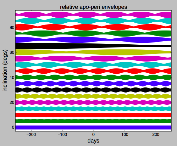
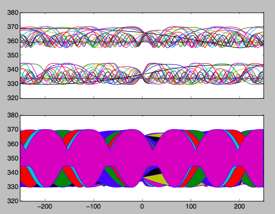
Tiangong-1 rough simulation

Tiangong-1 rough simulation

def make_fake_TLE(incdegs, ecc, altkm):
    "don't try this at home!!!"
    a          = (6378+altkm) * 1000.
    revsperday = 24.*3600/(twopi * np.sqrt(a**3 / GMe))

    eccstr = '{:07d}'.format(int(1E+07 * ecc))
    mmstr  = '{:011.8f}'.format(revsperday)
    incstr = '{:08.4f}'.format(incdegs)

    L1 = "1 00000x xxxxxx   17091.00000000 +.00000000 +00000-0 +00000-3 0  0000"
    L2 = "2 00000 " + incstr + " 000.0000 " + eccstr + " 000.0000 000.0000 " + mmstr + "000000"

    return (L1, L2)

import numpy as np
import matplotlib.pyplot as plt
from skyfield.api import Loader, Topos, EarthSatellite

# Real TLE for TianGong-1 for April 1, 2017
# "1 37820U 11053A   17091.81919743 +.00033376 +00000-0 +21646-3 0  9994"
# "2 37820 042.7591 306.4244 0019428 259.0955 165.0115 15.75087641315914"

twopi = 2.*np.pi
GMe   = 3.986E+14  # earth standard gravitational parameter
Re_km = 6378.

days    = np.arange(500) - 250
minutes = np.arange(120)

delta_inc = 5. # degrees
n_inc     = 19 
incdegs = delta_inc * np.arange(n_inc) 

### NOTE!  The first time you run, set calculate to True! It takes several minutes to
# propagate all of the orbits, then saves the result as a  .npy file
# Then, set calculate to False. Now you can play with plotting without
# doing any more calculations, so it's much much faster.
# https://matplotlib.org/gallery/lines_bars_and_markers/fill_between_demo.html

calculate = True
fname     = 'incgroups19x-250to+250'

if calculate:
    load = Loader('~/Documents/fishing/SkyData')  # avoids multiple copies of large files
    ts   = load.timescale()

    data    = load('de421.bsp')
    earth   = data['earth']
    ts      = load.timescale()
    incgroups = []
    for incdeg in incdegs: 
        rmins, rmaxs = [], []
        for day in days:
            if not day%100:
                print day,
            time    = ts.utc(2017, 4, day, 0, minutes)  # starting April 1, 2017
            L1, L2  = make_fake_TLE(incdeg, 0.0019, 350.)
            TG1     = EarthSatellite(L1, L2)
            TG1pos  = TG1.at(time).position.km
            r       = np.sqrt((TG1pos**2).sum(axis=0))
            rmins.append(r.min())
            rmaxs.append(r.max())
        rmins = np.array(rmins)
        rmaxs = np.array(rmaxs)
        incgroups.append([rmins, rmaxs])

    incgroups = np.array(incgroups)

    if fname:
        q = np.stack(incgroups)
        np.save(fname, q)
else:
    if fname[-4].lower() != '.npy':
        fname += '.npy'
    incgroups = np.load(fname)

groups = incgroups.copy()

# post-process it
dh = 40.
for i, thing in enumerate(groups):
    thing += dh*i
baseline = groups[0].mean()
groups   = delta_inc * (groups-baseline)/dh


if True:
    N         = len(groups)
    colors    = plt.rcParams['axes.prop_cycle'].by_key()['color']
    for i, (rmin, rmax) in enumerate(groups):
        c  = colors[i%len(colors)]
        dh = 40. * i
        plt.fill_between(days, rmin, rmax,
                         color=None, facecolor=c, linewidth=0)
    plt.xlim(-250, 250)
    plt.ylim(-3, 94)
    plt.xlabel('days', fontsize=16)
    plt.title('relative apo-peri envelopes', fontsize=16)
    plt.ylabel('inclination (degs)', fontsize=16)
    plt.show()

if True:
    colors = plt.rcParams['axes.prop_cycle'].by_key()['color']
    fig, (ax1, ax2) = plt.subplots(2, 1, sharex=True)
    for i, (rmin, rmax) in enumerate(incgroups):
        c = colors[i%len(colors)]
        ax1.plot(days, rmin-Re_km, c)
        ax1.plot(days, rmax-Re_km, c)
        ax2.fill_between(days, rmin-Re_km, rmax-Re_km, color='b', facecolor=c)
    ax1.set_xlim(-250, 250)
    ax2.set_xlim(-250, 250)
    plt.show()
$\endgroup$
7
  • 1
    $\begingroup$ The horizontal axis is the time in days, the vertical the orbit height in km. The different colors are for the 0, 20, 40, 60, and 80 degrees inclinations and for apogee and perigee? $\endgroup$
    – Uwe
    Commented May 2, 2018 at 10:11
  • 1
    $\begingroup$ @Uwe yes for all, thanks! I will run it again and add some labels tomorrow. $\endgroup$
    – uhoh
    Commented May 2, 2018 at 11:01
  • 1
    $\begingroup$ @Uwe well, it's not exactly "tomorrow" but I've updated the plots. Suggestions welcome! $\endgroup$
    – uhoh
    Commented Oct 9, 2018 at 4:09
  • 1
    $\begingroup$ @uhoh so is this an Earth-gravity perturbation? the period looks to me like it is related to the moon 3rd body effects. $\endgroup$
    – costrom
    Commented Jun 16, 2019 at 23:46
  • 1
    $\begingroup$ @costrom that's a good question. The calculation I did here uses SGP4, which does not apply any 3rd body effects to such low orbits. As a side note, SGP4 only has minimal, approximate corrections for high orbits. See the sentences above: "Since the period of this LEO is less than 225 minutes, SGP4 does not use the SDP4 "deep space" corrections for the Sun and Moon's gravity. So the only effect left is the Earth's gravitational field's departure from spherical." $\endgroup$
    – uhoh
    Commented Jun 16, 2019 at 23:53
6
$\begingroup$

After the uhoh's excellent answer, there’s no need for another answer, but with a simulation we can see the effect of the Earth's oblateness and of the atmosphere.

The simulation includes the Newtonian and the relativistic accelerations of all the planets, Sun and Moon.
The Earth's gravity field is modeled with the SGG-UGM-1 gravity model (computed using EGM2008 derived gravity anomaly and GOCE observation data) truncated to the degree and order 15 (to save the running time, while retaining good accuracy when compared to the full model).
For the calculation of the air density, I use the NRLMSISE-00 model along with an updated data file for the solar and geomagnetic indices. The actual indices can be found here: www.celestrak.com/spacedata/SW-All.txt.

The first step involves determining the best ballistic coefficient to minimize a particular simulation parameter. After 36 minutes, the program finds a ballistic coefficient of about $111\,kg/m^2$ (it’s not fixed, because the drag coefficient varies with the air composition).

Now the simulation can be started:
1) with one TLE and the CSpOC’s SGP4 propagator calculate the initial state (position and velocity) of the satellite for the TLE epoch;
2) propagate that initial state with a specially crafted propagator (my propagator is based on the 8(5,3) Dormand-Prince integrator);
3) when the satellite altitude drops below 70 km, stop the simulation.

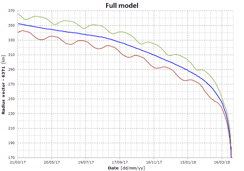
Here’s the result obtained with the TLE 17080.91114878:

full model

The graph shows that my model accurately reproduces the Wikipedia graph.


Why are the graphs wobbly? Is it because the Earth is not exactly a sphere and also due to uneven mass distribution?

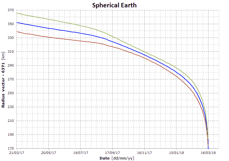
You can answer that question by simulating the Earth as if it were a sphere; here’s the result:

spherical Earth

The wobbling is no longer shown (we see an irregular decay rate because the air density varies according to solar activity).


Why are the graphs wobbly? Is it an atmospheric effect?

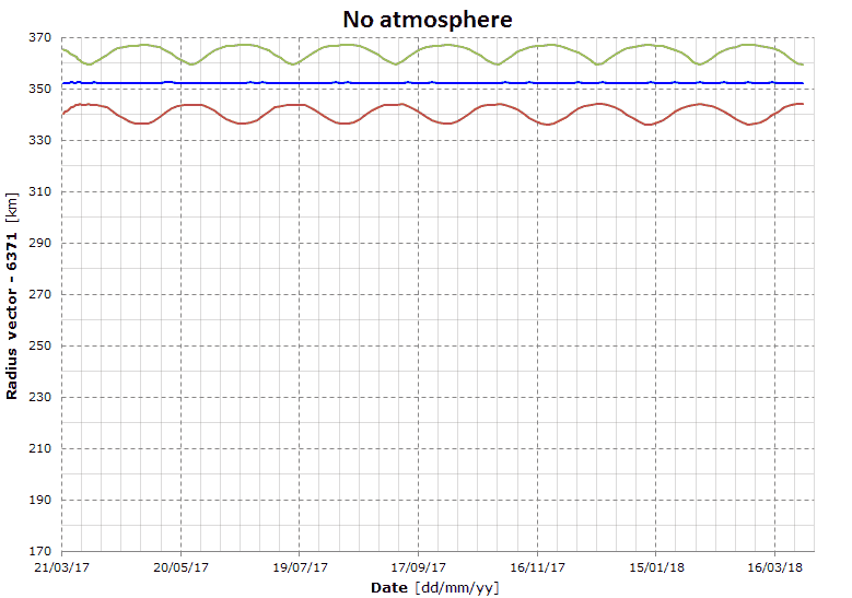
To answer that question we just need to disable the atmosphere; here’s the result:

no atmosphere

The wobbling is exactly the same as the full model.

$\endgroup$
0
$\begingroup$

Compared to other plots of the orbit the oscillation seems to be quite exaggerated.

Theories

I am no expert on this, but looking around a bit I have a few theories and found quit a bit of oscillations of altitudes and eccentricities for space stations.

Nodal precession

I think it is due to the nodal precession of the station the period is about two months for the ISS, I think it would be similar for Tiangong. I found this while looking at this answer. Nodal precession is the inclination of the station oscillating due to the earth not being a sphere.

Then I’d expect the average altitude of the station to go down with low inclinations and up with high ones. That however does not fully explain why Apogee and Perigee are opposed to each other on this one.

That is wrong. Thanks to @M.A.H. For catching that one. Stupid me looked it up / remembered it wrong.

Lunar resonance

It might also be due to some sort of lunar influence with those two months, but just a guess.

Different oscillations

14 day eccentricity resonance

On the nasaspaceflight forums they found a slower oscillation, which might be related.

Half orbit

Another, much more small scale oscillation, wich you can see in the image below in the top right is actually due to the oblatenes of the earth. The altitude decreases every time over the equator which is thicker than the rest of the earth. alt source

$\endgroup$
5
  • 1
    $\begingroup$ Nodal procession is the procession of the RAAN, not the inclination. $\endgroup$
    – M.A.H.
    Commented Apr 1, 2018 at 23:14
  • $\begingroup$ Oh, sh*t, whoops, thanks, didn’t look deep enough/ just read the wrong parts, thanks! $\endgroup$
    – Hans
    Commented Apr 1, 2018 at 23:19
  • $\begingroup$ The effect due to the oblateness shows up twice per orbit (one every 45 minutes or so) The eccentricity shows up once per orbit (every 90 minutes or so) Most of the Aerospace Corp image seems to be eccentricity. $\endgroup$ Commented Apr 2, 2018 at 1:32
  • $\begingroup$ So is this lunar effect ? If so, period should be one month right? But it seems period is two months. $\endgroup$
    – zephyr0110
    Commented Apr 4, 2018 at 9:13
  • $\begingroup$ You missed apsidal precession. Perigee altitude will increase (decrease) as perigee moves away from (toward) the equator due to the Earth's equatorial bulge. $\endgroup$ Commented Dec 30, 2019 at 19:53

Your Answer

By clicking “Post Your Answer”, you agree to our terms of service and acknowledge you have read our privacy policy.

Not the answer you're looking for? Browse other questions tagged or ask your own question.